

Cross-Gyre Flow
279
5.2 Cross-Gyre Flow
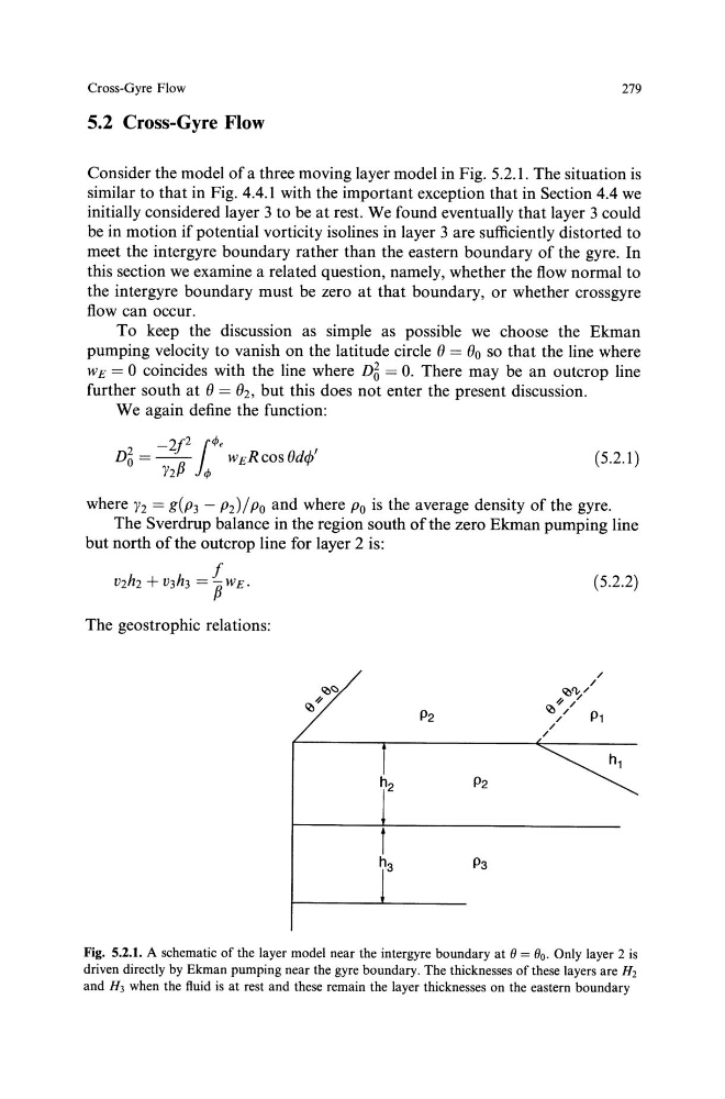
Consider the model of a three moving layer model in Fig. 5.2.1. The situation is
similar to that in Fig. 4.4.1 with the important exception that in Section 4.4 we
initially considered layer 3 to be at rest. We found eventually that layer 3 could
be in motion if potential vorticity isolines in layer 3 are sufficiently distorted to
meet the intergyre boundary rather than the eastern boundary of the gyre. In
this section we examine a related question, namely, whether the flow normal to
the intergyre boundary must be zero at that boundary, or whether crossgyre
flow can occur.
To keep the discussion as simple as possible we choose the Ekman
pumping velocity to vanish on the latitude circle e = eo so that the line where
WE= 0 coincides with the line where D6 = 0. There may be an outcrop line
further south at e = e2, but this does not enter the present discussion.
We again define the function:
-2P1"''
D~ = - 13 -
w ER cos 8dcp'
Y2
q,
( 5.2.1)
where y2 = g(p 3 - p 2 )/ Po and where Po is the average density of the gyre.
The Sverdrup balance in the region south of the zero Ekman pumping line
but north of the outcrop line for layer 2 is:
f
v2h2 + v3h3 = PW£.
(5.2.2)
The geostrophic relations:
P3
Fig. 5.2.1. A schematic of the layer model near the intergyre boundary at e = 00• Only layer 2 is
driven directly by Ekman pumping near the gyre boundary. The thicknesses of these layers are H 2
and H3 when the fluid is at rest and these remain the layer thicknesses on the eastern boundary
279
5.2 Cross-Gyre Flow
Consider the model of a three moving layer model in Fig. 5.2.1. The situation is
similar to that in Fig. 4.4.1 with the important exception that in Section 4.4 we
initially considered layer 3 to be at rest. We found eventually that layer 3 could
be in motion if potential vorticity isolines in layer 3 are sufficiently distorted to
meet the intergyre boundary rather than the eastern boundary of the gyre. In
this section we examine a related question, namely, whether the flow normal to
the intergyre boundary must be zero at that boundary, or whether crossgyre
flow can occur.
To keep the discussion as simple as possible we choose the Ekman
pumping velocity to vanish on the latitude circle e = eo so that the line where
WE= 0 coincides with the line where D6 = 0. There may be an outcrop line
further south at e = e2, but this does not enter the present discussion.
We again define the function:
-2P1"''
D~ = - 13 -
w ER cos 8dcp'
Y2
q,
( 5.2.1)
where y2 = g(p 3 - p 2 )/ Po and where Po is the average density of the gyre.
The Sverdrup balance in the region south of the zero Ekman pumping line
but north of the outcrop line for layer 2 is:
f
v2h2 + v3h3 = PW£.
(5.2.2)
The geostrophic relations:
P3
Fig. 5.2.1. A schematic of the layer model near the intergyre boundary at e = 00• Only layer 2 is
driven directly by Ekman pumping near the gyre boundary. The thicknesses of these layers are H 2
and H3 when the fluid is at rest and these remain the layer thicknesses on the eastern boundary