

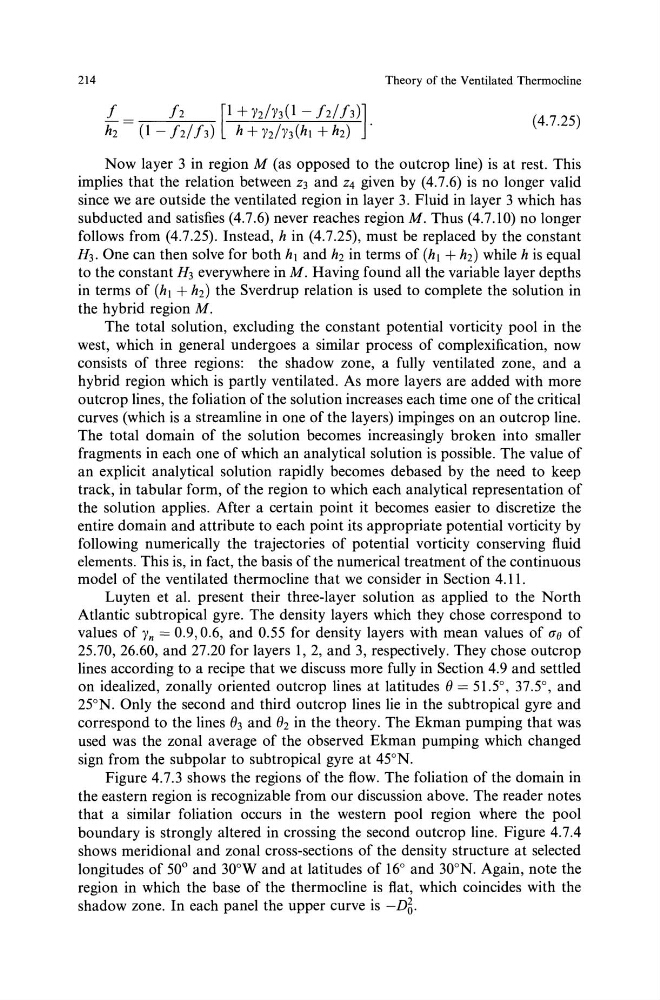
214
Theory of the Ventilated Thermocline
Now layer 3 in region M (as opposed to the outcrop line) is at rest. This
implies that the relation between z3 and z4 given by (4.7.6) is no longer valid
since we are outside the ventilated region in layer 3. Fluid in layer 3 which has
subducted and satisfies (4.7.6) never reaches region M. Thus (4.7.10) no longer
follows from (4.7.25). Instead, h in (4.7.25), must be replaced by the constant
H3. One can then solve for both h1 and hz in terms of (h 1 + hz) while his equal
to the constant H 3 everywhere in M. Having found all the variable layer depths
in terms of (h 1 + h2) the Sverdrup relation is used to complete the solution in
the hybrid region M.
The total solution, excluding the constant potential vorticity pool in the
west, which in general undergoes a similar process of complexification, now
consists of three regions: the shadow zone, a fully ventilated zone, and a
hybrid region which is partly ventilated. As more layers are added with more
outcrop lines, the foliation ofthe solution increases each time one of the critical
curves (which is a streamline in one of the layers) impinges on an outcrop line.
The total domain of the solution becomes increasingly broken into smaller
fragments in each one of which an analytical solution is possible. The value of
an explicit analytical solution rapidly becomes debased by the need to keep
track, in tabular form, of the region to which each analytical representation of
the solution applies. After a certain point it becomes easier to discretize the
entire domain and attribute to each point its appropriate potential vorticity by
following numerically the trajectories of potential vorticity conserving fluid
elements. This is, in fact, the basis of the numerical treatment of the continuous
model of the ventilated thermocline that we consider in Section 4.11.
Luyten et al. present their three-layer solution as applied to the North
Atlantic subtropical gyre. The density layers which they chose correspond to
values of Yn = 0.9, 0.6, and 0.55 for density layers with mean values of uo of
25.70, 26.60, and 27.20 for layers 1, 2, and 3, respectively. They chose outcrop
lines according to a recipe that we discuss more fully in Section 4.9 and settled
on idealized, zonally oriented outcrop lines at latitudes (} = 51 .SO, 37 .SO, and
25°N. Only the second and third outcrop lines lie in the subtropical gyre and
correspond to the lines (}3 and (}2 in the theory. The Ekman pumping that was
used was the zonal average of the observed Ekman pumping which changed
sign from the subpolar to subtropical gyre at 45°N.
Figure 4.7.3 shows the regions of the flow. The foliation of the domain in
the eastern region is recognizable from our discussion above. The reader notes
that a similar foliation occurs in the western pool region where the pool
boundary is strongly altered in crossing the second outcrop line. Figure 4. 7.4
shows meridional and zonal cross-sections of the density structure at selected
longitudes of 50° and 30°W and at latitudes of 16° and 30°N. Again, note the
region in which the base of the thermocline is flat, which coincides with the
shadow zone. In each panel the upper curve is -D6.
Theory of the Ventilated Thermocline
Now layer 3 in region M (as opposed to the outcrop line) is at rest. This
implies that the relation between z3 and z4 given by (4.7.6) is no longer valid
since we are outside the ventilated region in layer 3. Fluid in layer 3 which has
subducted and satisfies (4.7.6) never reaches region M. Thus (4.7.10) no longer
follows from (4.7.25). Instead, h in (4.7.25), must be replaced by the constant
H3. One can then solve for both h1 and hz in terms of (h 1 + hz) while his equal
to the constant H 3 everywhere in M. Having found all the variable layer depths
in terms of (h 1 + h2) the Sverdrup relation is used to complete the solution in
the hybrid region M.
The total solution, excluding the constant potential vorticity pool in the
west, which in general undergoes a similar process of complexification, now
consists of three regions: the shadow zone, a fully ventilated zone, and a
hybrid region which is partly ventilated. As more layers are added with more
outcrop lines, the foliation ofthe solution increases each time one of the critical
curves (which is a streamline in one of the layers) impinges on an outcrop line.
The total domain of the solution becomes increasingly broken into smaller
fragments in each one of which an analytical solution is possible. The value of
an explicit analytical solution rapidly becomes debased by the need to keep
track, in tabular form, of the region to which each analytical representation of
the solution applies. After a certain point it becomes easier to discretize the
entire domain and attribute to each point its appropriate potential vorticity by
following numerically the trajectories of potential vorticity conserving fluid
elements. This is, in fact, the basis of the numerical treatment of the continuous
model of the ventilated thermocline that we consider in Section 4.11.
Luyten et al. present their three-layer solution as applied to the North
Atlantic subtropical gyre. The density layers which they chose correspond to
values of Yn = 0.9, 0.6, and 0.55 for density layers with mean values of uo of
25.70, 26.60, and 27.20 for layers 1, 2, and 3, respectively. They chose outcrop
lines according to a recipe that we discuss more fully in Section 4.9 and settled
on idealized, zonally oriented outcrop lines at latitudes (} = 51 .SO, 37 .SO, and
25°N. Only the second and third outcrop lines lie in the subtropical gyre and
correspond to the lines (}3 and (}2 in the theory. The Ekman pumping that was
used was the zonal average of the observed Ekman pumping which changed
sign from the subpolar to subtropical gyre at 45°N.
Figure 4.7.3 shows the regions of the flow. The foliation of the domain in
the eastern region is recognizable from our discussion above. The reader notes
that a similar foliation occurs in the western pool region where the pool
boundary is strongly altered in crossing the second outcrop line. Figure 4. 7.4
shows meridional and zonal cross-sections of the density structure at selected
longitudes of 50° and 30°W and at latitudes of 16° and 30°N. Again, note the
region in which the base of the thermocline is flat, which coincides with the
shadow zone. In each panel the upper curve is -D6.