

Determination of the Recirculation
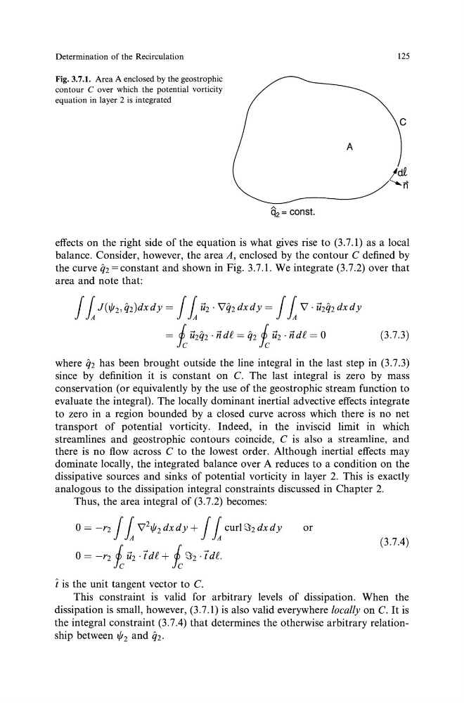
Fig. 3.7.1. Area A enclosed by the geostrophic
contour C over which the potential vorticity
equation in layer 2 is integrated
125
cb= canst.
effects on the right side of the equation is what gives rise to (3.7.1) as a local
balance. Consider, however, the area A, enclosed by the contour C defined by
the curve q2 =constant and shown in Fig. 3.7.1. We integrate (3.7.2) over that
area and note that:
J 1 J(l/12.?1z)dxdy = J 1 i12 · '\lq2 dxdy = J 1 '\1 · i1zq2 dxdy
= i i12q2 · ii dl = qz i i12 · ii dl = 0
(3.7.3)
where q2 has been brought outside the line integral in the last step in (3.7.3)
since by definition it is constant on C. The last integral is zero by mass
conservation (or equivalently by the use of the geostrophic stream function to
evaluate the integral). The locally dominant inertial advective effects integrate
to zero in a region bounded by a closed curve across which there is no net
transport of potential vorticity. Indeed, in the inviscid limit in which
streamlines and geostrophic contours coincide, C is also a streamline, and
there is no flow across C to the lowest order. Although inertial effects may
dominate locally, the integrated balance over A reduces to a condition on the
dissipative sources and sinks of potential vorticity in layer 2. This is exactly
analogous to the dissipation integral constraints discussed in Chapter 2.
Thus, the area integral of (3.7.2) becomes:
0 = -r2 J 1 '\1 2 ljl2dxdy+ J 1 curl~2dxdy
0 = -r2 i i12 · 7 dl + i ~2 · 7 dl.
t is the unit tangent vector to C.
or
(3.7.4)
This constraint is valid for arbitrary levels of dissipation. When the
dissipation is small, however, (3.7.1) is also valid everywhere locally on C. It is
the integral constraint (3.7.4) that determines the otherwise arbitrary relationship between l /1 2 and q2.
Fig. 3.7.1. Area A enclosed by the geostrophic
contour C over which the potential vorticity
equation in layer 2 is integrated
125
cb= canst.
effects on the right side of the equation is what gives rise to (3.7.1) as a local
balance. Consider, however, the area A, enclosed by the contour C defined by
the curve q2 =constant and shown in Fig. 3.7.1. We integrate (3.7.2) over that
area and note that:
J 1 J(l/12.?1z)dxdy = J 1 i12 · '\lq2 dxdy = J 1 '\1 · i1zq2 dxdy
= i i12q2 · ii dl = qz i i12 · ii dl = 0
(3.7.3)
where q2 has been brought outside the line integral in the last step in (3.7.3)
since by definition it is constant on C. The last integral is zero by mass
conservation (or equivalently by the use of the geostrophic stream function to
evaluate the integral). The locally dominant inertial advective effects integrate
to zero in a region bounded by a closed curve across which there is no net
transport of potential vorticity. Indeed, in the inviscid limit in which
streamlines and geostrophic contours coincide, C is also a streamline, and
there is no flow across C to the lowest order. Although inertial effects may
dominate locally, the integrated balance over A reduces to a condition on the
dissipative sources and sinks of potential vorticity in layer 2. This is exactly
analogous to the dissipation integral constraints discussed in Chapter 2.
Thus, the area integral of (3.7.2) becomes:
0 = -r2 J 1 '\1 2 ljl2dxdy+ J 1 curl~2dxdy
0 = -r2 i i12 · 7 dl + i ~2 · 7 dl.
t is the unit tangent vector to C.
or
(3.7.4)
This constraint is valid for arbitrary levels of dissipation. When the
dissipation is small, however, (3.7.1) is also valid everywhere locally on C. It is
the integral constraint (3.7.4) that determines the otherwise arbitrary relationship between l /1 2 and q2.