

122
Vertical Structure: Baroclinic Quasi-Geostrophic Models
A
f3 [ 2 2 2 (
)2]
q2 = 2 Yo r 1 +Yo - x - Y- Yo
r < r,.
(3.6.7)
The isolines of q2, which within the disk are arcs of circles centered on y = Yo,
are lines of constant latitude outside the disk. For weak forcing (small IX) Yo is
greater than r1, and the geostrophic contours remain open. Each circular arc
within the disk connects to a geostrophic contour outside the disk, which is a
line of constant y. Each contour then strikes the eastern boundary, and the
motion on the contour is therefore blocked, and layer 2 remains at rest. Figure
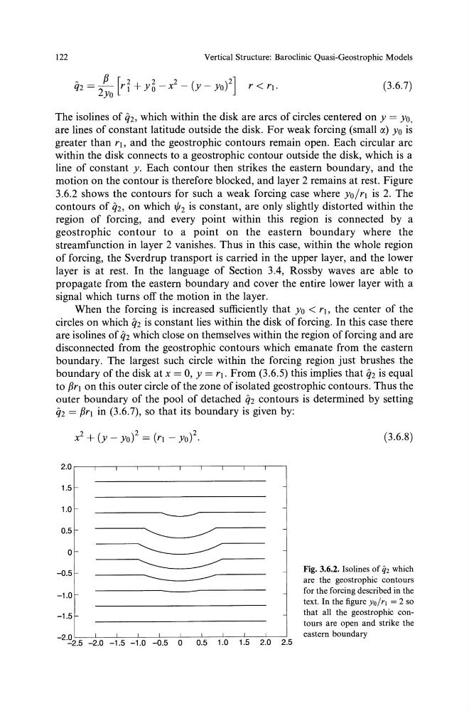
3.6.2 shows the contours for such a weak forcing case where yofr, is 2. The
contours of q2, on which t/1 2 is constant, are only slightly distorted within the
region of forcing, and every point within this region is connected by a
geostrophic contour to a point on the eastern boundary where the
streamfunction in layer 2 vanishes. Thus in this case, within the whole region
of forcing, the Sverdrup transport is carried in the upper layer, and the lower
layer is at rest. In the language of Section 3.4, Rossby waves are able to
propagate from the eastern boundary and cover the entire lower layer with a
signal which turns off the motion in the layer.
When the forcing is increased sufficiently that y0 < r1, the center of the
circles on which q2 is constant lies within the disk of forcing. In this case there
are isolines of q2 which close on themselves within the region of forcing and are
disconnected from the geostrophic contours which emanate from the eastern
boundary. The largest such circle within the forcing region just brushes the
boundary of the disk at x = 0, y = r,. From (3.6.5) this implies that q2 is equal
to f3r1 on this outer circle of the zone of isolated geostrophic contours. Thus the
outer boundary of the pool of detached q2 contours is determined by setting
q2 = f3r1 in (3.6.7), so that its boundary is given by:
2.0 ,------,---,------,---,-----.------,---,---,-----,-----,
1.5
1.0
0.5
0
-Q.5
-1.0
-1.5
- 2 -~2.5 -2.0 -1.5 -1.0 -o.5 0 0.5 1.0 1.5 2.0 2.5
(3.6.8)
Fig. 3.6.2. lsolines of f/2 which
are the geostrophic contours
for the forcing described in the
text. In the figure Yo/r1 = 2 so
that all the geostrophic contours are open and strike the
eastern boundary
Vertical Structure: Baroclinic Quasi-Geostrophic Models
A
f3 [ 2 2 2 (
)2]
q2 = 2 Yo r 1 +Yo - x - Y- Yo
r < r,.
(3.6.7)
The isolines of q2, which within the disk are arcs of circles centered on y = Yo,
are lines of constant latitude outside the disk. For weak forcing (small IX) Yo is
greater than r1, and the geostrophic contours remain open. Each circular arc
within the disk connects to a geostrophic contour outside the disk, which is a
line of constant y. Each contour then strikes the eastern boundary, and the
motion on the contour is therefore blocked, and layer 2 remains at rest. Figure
3.6.2 shows the contours for such a weak forcing case where yofr, is 2. The
contours of q2, on which t/1 2 is constant, are only slightly distorted within the
region of forcing, and every point within this region is connected by a
geostrophic contour to a point on the eastern boundary where the
streamfunction in layer 2 vanishes. Thus in this case, within the whole region
of forcing, the Sverdrup transport is carried in the upper layer, and the lower
layer is at rest. In the language of Section 3.4, Rossby waves are able to
propagate from the eastern boundary and cover the entire lower layer with a
signal which turns off the motion in the layer.
When the forcing is increased sufficiently that y0 < r1, the center of the
circles on which q2 is constant lies within the disk of forcing. In this case there
are isolines of q2 which close on themselves within the region of forcing and are
disconnected from the geostrophic contours which emanate from the eastern
boundary. The largest such circle within the forcing region just brushes the
boundary of the disk at x = 0, y = r,. From (3.6.5) this implies that q2 is equal
to f3r1 on this outer circle of the zone of isolated geostrophic contours. Thus the
outer boundary of the pool of detached q2 contours is determined by setting
q2 = f3r1 in (3.6.7), so that its boundary is given by:
2.0 ,------,---,------,---,-----.------,---,---,-----,-----,
1.5
1.0
0.5
0
-Q.5
-1.0
-1.5
- 2 -~2.5 -2.0 -1.5 -1.0 -o.5 0 0.5 1.0 1.5 2.0 2.5
(3.6.8)
Fig. 3.6.2. lsolines of f/2 which
are the geostrophic contours
for the forcing described in the
text. In the figure Yo/r1 = 2 so
that all the geostrophic contours are open and strike the
eastern boundary