

World Ocean Circulation Experiment
187
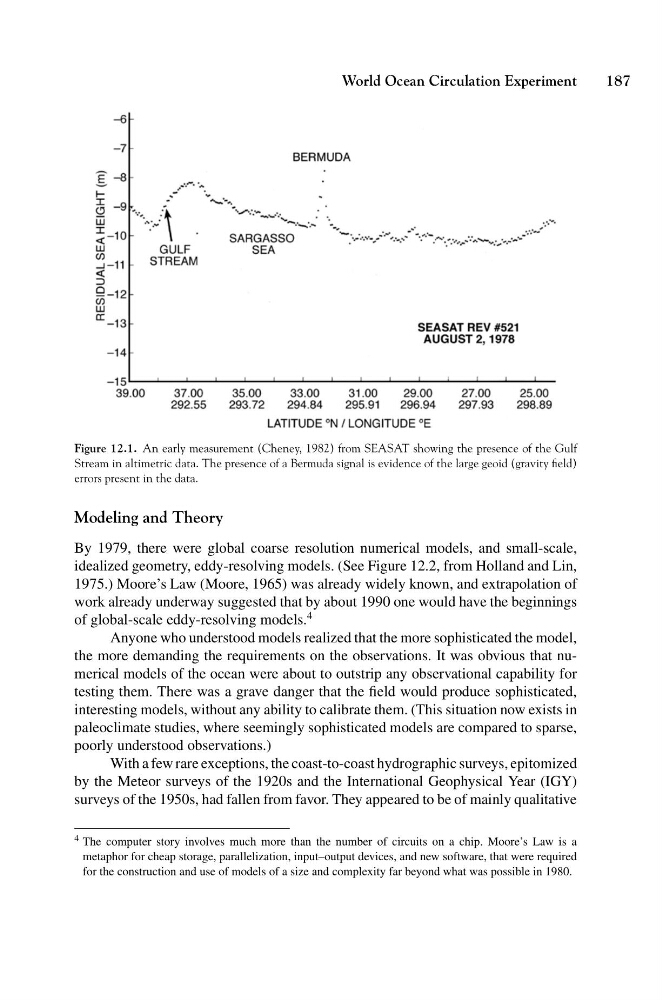
Figure 12.1. An early measurement (Cheney, 1982) from SEASAT showing the presence of the Gulf
Stream in altimetric data. The presence of a Bermuda signal is evidence of the large geoid (gravity field)
errors present in the data.
Modeling and Theory
By 1979, there were global coarse resolution numerical models, and small-scale,
idealized geometry, eddy-resolving models. (See Figure 12.2, from Holland and Lin,
1975.) Moore’s Law (Moore, 1965) was already widely known, and extrapolation of
work already underway suggested that by about 1990 one would have the beginnings
of global-scale eddy-resolving models.
4
Anyone who understood models realized that the more sophisticated the model,
the more demanding the requirements on the observations. It was obvious that numerical models of the ocean were about to outstrip any observational capability for
testing them. There was a grave danger that the field would produce sophisticated,
interesting models, without any ability to calibrate them. (This situation now exists in
paleoclimate studies, where seemingly sophisticated models are compared to sparse,
poorly understood observations.)
With a few rare exceptions, the coast-to-coast hydrographic surveys, epitomized
by the Meteor surveys of the 1920s and the International Geophysical Year (IGY)
surveys of the 1950s, had fallen from favor. They appeared to be of mainly qualitative
4 The computer story involves much more than the number of circuits on a chip. Moore’s Law is a
metaphor for cheap storage, parallelization, input–output devices, and new software, that were required
for the construction and use of models of a size and complexity far beyond what was possible in 1980.
187
Figure 12.1. An early measurement (Cheney, 1982) from SEASAT showing the presence of the Gulf
Stream in altimetric data. The presence of a Bermuda signal is evidence of the large geoid (gravity field)
errors present in the data.
Modeling and Theory
By 1979, there were global coarse resolution numerical models, and small-scale,
idealized geometry, eddy-resolving models. (See Figure 12.2, from Holland and Lin,
1975.) Moore’s Law (Moore, 1965) was already widely known, and extrapolation of
work already underway suggested that by about 1990 one would have the beginnings
of global-scale eddy-resolving models.
4
Anyone who understood models realized that the more sophisticated the model,
the more demanding the requirements on the observations. It was obvious that numerical models of the ocean were about to outstrip any observational capability for
testing them. There was a grave danger that the field would produce sophisticated,
interesting models, without any ability to calibrate them. (This situation now exists in
paleoclimate studies, where seemingly sophisticated models are compared to sparse,
poorly understood observations.)
With a few rare exceptions, the coast-to-coast hydrographic surveys, epitomized
by the Meteor surveys of the 1920s and the International Geophysical Year (IGY)
surveys of the 1950s, had fallen from favor. They appeared to be of mainly qualitative
4 The computer story involves much more than the number of circuits on a chip. Moore’s Law is a
metaphor for cheap storage, parallelization, input–output devices, and new software, that were required
for the construction and use of models of a size and complexity far beyond what was possible in 1980.