

Reconstructing and Modelling the Last Glacial Maximum
701
:lC('· .... 1
a ) measured (km)
b) modelled (km )
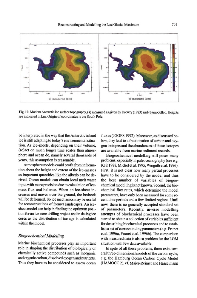
Fig. 10. ModemAntarctic ice surface topography, (a) measured as given by Drewry (1983) and (b) modelled. Heights
are indicated in km. Origin of coordinates is the South Pole.
be interpreted in the way that the Antarctic inland
ice is still adapting to today's environmental situation. As ice-sheets, depending on their volume,
(re)act on much longer time scales than atmosphere and ocean do, namely several thousands of
years, this assumption is reasonable.
Atmosphere models could profit from information about the height and extent of the ice-masses
as important quantities like the albedo can be derived. Ocean models can obtain local melt water
input with more precision due to calculation of icemass flux and balance. When an ice-sheet increases and moves over the ground, the bedrock
will be deformed. So ice mechanics may be useful
for reconstructions of former landscapes. An icesheet model can help in finding the optimum position for an ice-core drilling project and in dating ice
cores as the distribution of ice age is calculated
within the model.
Biogeochemical Modelling
Marine biochemical processes play an important
role in shaping the distribution of biologically or
chemically active compounds such as inorganic
and organic carbon, dissolved oxygen and nutrients.
Thus they have to be considered to assess ocean
fluxes (JGOFS 1992). Moreover, as discussed below, they lead to a fractionation of carbon and oxygen isotopes and the abundances ofthese isotopes
are available from marine sediment records.
Biogeochemical modelling still poses many
problems, especially in paleoceanography (see e.g.
Keir 1988, Michel etal. 1995, Winguthetal. 1996).
First, it is not clear how many partial processes
have to be considered by the model and thus
the best number of variables of biogeochemical modelling is not known. Second, the biochemical flux rates, which determine the model
parameters, have only been measured for some recent time periods and a few limited regions. Until
now, there is no generally accepted standard set
of parameters. Recently, inverse modelling
attempts of biochemical processes have been
started to obtain a collection of variables sufficient
for describing biochemical processes and to establish a set of corresponding parameters (e.g. Prunet
et al. 1996a, Prunet et al. 1996b). The comparison
with measured data is also a problem for the LGM
situation with few data available.
In spite of all these problems, there exist several three-dimensional models of the carbon cycle,
e.g. the Hamburg Ocean Carbon Cycle Model
(HAMOCC 2), cf. Maier-Reimer and Hasselmann