

On the Reconstruction of Paleo salinities
211
Application to Core-Top Data
We computed salinities for a global data set of coretop isotopic measurements. Data have been collected from the literature (references are summarized in Table 1). The data set comprises 777 measurements from high to low latitudes in all major
oceans with a large number of samples in the Atlantic and Indian Oceans, and only a few in the
Pacific. Isotopic data from four shallow-dwelling
planktonic foraminifera G. ruber, G. sacculifer, G.
bulloides and N. pachyderma have been used.
The data were not selected according to the size
fractions of analyzed foraminifera or the number
of individuals measured in one sample. Distinctions
between G. ruber (white) and G. ruber (pink)
were not made here.
In the first step, 1) 18 0 of sea-water was calculated by inserting annual mean temperatures for all
sample locations in equation (2). Temperatures
were taken from the W orId Ocean Atlas 1994
(Levitus and Boyer 1994). Calibrations according
to equation (3) were not applied. In the second step,
annual mean salinities were computed by inserting
the SMOW-corrected sea-water 1) 18 0 into equation (7). A global 1) 18 0 w -saiinity relationship was
used (a = 0.5, b = 17), corrections for ice effects
are, of course, not necessary for the modem ocean.
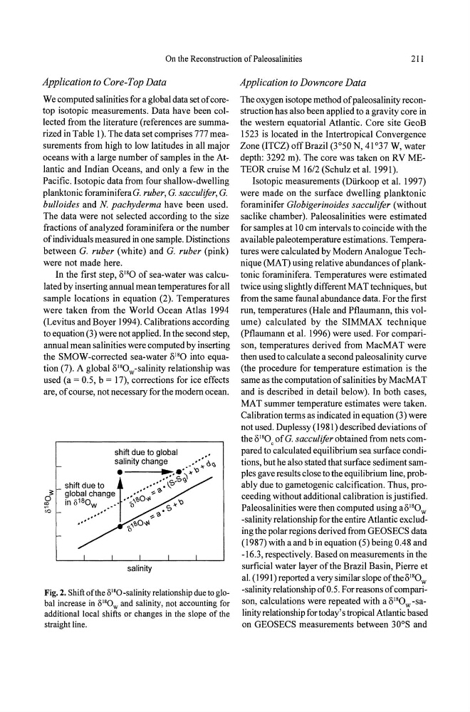
salinity
Fig. 2. Shift of the 0 18 0 -salinity relationship due to global increase in 0180 W and salinity, not accounting for
additional local shifts or changes in the slope of the
straight line.
Application to Downcore Data
The oxygen isotope method of paleosalinity reconstruction has also been applied to a gravity core in
the western equatorial Atlantic. Core site GeoB
1523 is located in the Intertropical Convergence
Zone (ITCZ) off Brazil (3°50 N, 41°37 W, water
depth: 3292 m). The core was taken on RV METEOR cruise M 16/2 (Schulz et al. 1991).
Isotopic measurements (Dlirkoop et al. 1997)
were made on the surface dweIling planktonic
foraminifer Globigerinoides sacculifer (without
saclike chamber). Paleosalinities were estimated
for samples at 10 em intervals to coincide with the
available paleotemperature estimations. Temperatures were calculated by Modem Analogue Technique (MAT) using relative abundances of planktonic foraminifera. Temperatures were estimated
twice using slightly different MAT techniques, but
from the same faunal abundance data. For the first
run, temperatures (Hale and Pflaumann, this volume) calculated by the SIMMAX technique
(Pflaumann et al. 1996) were used. For comparison, temperatures derived from MacMAT were
then used to calculate a second paleosalinity curve
(the procedure for temperature estimation is the
same as the computation of salinities by MacMA T
and is described in detail below). In both cases,
MAT summer temperature estimates were taken.
Calibration terms as indicated in equation (3) were
not used. Duplessy (1981) described deviations of
the 0180 c ofG. sacculifer obtained from nets compared to calculated equilibrium sea surface conditions, but he also stated that surface sediment samples gave results close to the equilibrium line, probably due to gametogenic calcification. Thus, proceeding without additional calibration is justified.
Paleosalinities were then computed using ao l8 0 w
-salinity relationship for the entire Atlantic excludingthepolarregions derived from GEOSECS data
(1987) with a and b in equation (5) being 0.48 and
-16.3, respectively. Based on measurements in the
surficial water layer of the Brazil Basin, Pierre et
al. (199 I) reported a very similar slope of the 0180 W
-salinity relationship of 0.5 . Forreasons of comparison, calculations were repeated with a 0180 w -salinity relationship for today' s tropical Atlantic based
on GEOSECS measurements between 30 0 S and
211
Application to Core-Top Data
We computed salinities for a global data set of coretop isotopic measurements. Data have been collected from the literature (references are summarized in Table 1). The data set comprises 777 measurements from high to low latitudes in all major
oceans with a large number of samples in the Atlantic and Indian Oceans, and only a few in the
Pacific. Isotopic data from four shallow-dwelling
planktonic foraminifera G. ruber, G. sacculifer, G.
bulloides and N. pachyderma have been used.
The data were not selected according to the size
fractions of analyzed foraminifera or the number
of individuals measured in one sample. Distinctions
between G. ruber (white) and G. ruber (pink)
were not made here.
In the first step, 1) 18 0 of sea-water was calculated by inserting annual mean temperatures for all
sample locations in equation (2). Temperatures
were taken from the W orId Ocean Atlas 1994
(Levitus and Boyer 1994). Calibrations according
to equation (3) were not applied. In the second step,
annual mean salinities were computed by inserting
the SMOW-corrected sea-water 1) 18 0 into equation (7). A global 1) 18 0 w -saiinity relationship was
used (a = 0.5, b = 17), corrections for ice effects
are, of course, not necessary for the modem ocean.
salinity
Fig. 2. Shift of the 0 18 0 -salinity relationship due to global increase in 0180 W and salinity, not accounting for
additional local shifts or changes in the slope of the
straight line.
Application to Downcore Data
The oxygen isotope method of paleosalinity reconstruction has also been applied to a gravity core in
the western equatorial Atlantic. Core site GeoB
1523 is located in the Intertropical Convergence
Zone (ITCZ) off Brazil (3°50 N, 41°37 W, water
depth: 3292 m). The core was taken on RV METEOR cruise M 16/2 (Schulz et al. 1991).
Isotopic measurements (Dlirkoop et al. 1997)
were made on the surface dweIling planktonic
foraminifer Globigerinoides sacculifer (without
saclike chamber). Paleosalinities were estimated
for samples at 10 em intervals to coincide with the
available paleotemperature estimations. Temperatures were calculated by Modem Analogue Technique (MAT) using relative abundances of planktonic foraminifera. Temperatures were estimated
twice using slightly different MAT techniques, but
from the same faunal abundance data. For the first
run, temperatures (Hale and Pflaumann, this volume) calculated by the SIMMAX technique
(Pflaumann et al. 1996) were used. For comparison, temperatures derived from MacMAT were
then used to calculate a second paleosalinity curve
(the procedure for temperature estimation is the
same as the computation of salinities by MacMA T
and is described in detail below). In both cases,
MAT summer temperature estimates were taken.
Calibration terms as indicated in equation (3) were
not used. Duplessy (1981) described deviations of
the 0180 c ofG. sacculifer obtained from nets compared to calculated equilibrium sea surface conditions, but he also stated that surface sediment samples gave results close to the equilibrium line, probably due to gametogenic calcification. Thus, proceeding without additional calibration is justified.
Paleosalinities were then computed using ao l8 0 w
-salinity relationship for the entire Atlantic excludingthepolarregions derived from GEOSECS data
(1987) with a and b in equation (5) being 0.48 and
-16.3, respectively. Based on measurements in the
surficial water layer of the Brazil Basin, Pierre et
al. (199 I) reported a very similar slope of the 0180 W
-salinity relationship of 0.5 . Forreasons of comparison, calculations were repeated with a 0180 w -salinity relationship for today' s tropical Atlantic based
on GEOSECS measurements between 30 0 S and