

Part A | 2.8
42 Part A Fundamentals
phase (Ä i ) for each of the partial tides (or tidal constituents Á i with its own ! i / given by
Á i D H i cos.! i t C Ä i / :
The harmonic constant H i =Ä i pairs for each of the partial tides can be obtained by a harmonic analysis of
a sufficiently long measured record – in this case sea
level SL.t/ – from the site of interest. Modern harmonic
analyses of measured records are based on a spectral
Computed
Observed
0
4
8
1 2
1 6
2 0
2 4
K 2
K 1
N 2
P 1
O 1
S 2
M 2
K 1
K 2
N 2
P 1
O 1
S 2
S 2
M 2
M 2
a)
b)
Time (h)
30
20
10
0
–10
–20
–30
–40
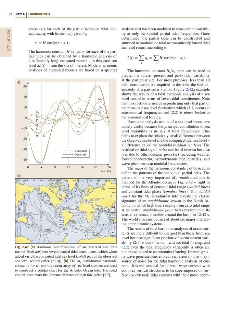
Fig. 2.42 (a) Harmonic decomposition of an observed sea level
record (dash-dot) into several partial tidal constituents, which when
added yield the computed tidal sea level (solid) part of the observed
sea level record (after [2.10]). (b) The M 2 semidiurnal harmonic
constants for an world’s ocean array of sea level stations are used
to construct a cotidal chart for the Atlantic Ocean tide. The solid
cotidal lines mark the Greenwich times of high tide (after [2.7])
analysis that has been modified to consider the variability at only the special partial tidal frequencies. Once
determined, the partial tides can be constructed and
summed to produce the total astronomically forced tidal
sea level record according to
h.t/ D
X
i
Á i D
X
i
H i cos.! i t C Ä i / :
The harmonic constant H i =Ä i pairs can be used to
predict the future (present and past) tidal variability
at the particular site. For most purposes, less than 10
tidal constituents are required to describe the tide adequately at a particular station. Figure 2.42a example
shows the results of a tidal harmonic analysis of a sea
level record in terms of seven tidal constituents. Note
that this method is useful in predicting only that part of
the measured sea level fluctuation which (2.1) occurs at
astronomical frequencies and (2.2) is phase locked to
the astronomical forcing.
Harmonic analysis results of a sea level record are
widely useful because the principal contribution to sea
level variability is usually at tidal frequencies. This
helps to explain the relatively small difference between
the observed sea level and the computed tidal sea level –
a difference called the nontidal residual sea level. The
residual or tidal signal noise can be of interest because
it is due to other oceanic processes including weather
forced phenomena, hydrodynamic nonlinearities, and
wave phenomena at nontidal frequencies.
The maps of the harmonic constants can be used to
define the patterns of the individual partial tides. The
pattern of the very important M 2 semidiurnal tide is
mapped for the Atlantic ocean in Fig. 2.42 – right in
terms of its lines of constant tidal range (cotidal lines)
and constant tidal phase (copahse lines). This cotidal
chart for the M 2 semidiurnal tide reveals the classic
signature of an amphidromic system in the North Atlantic; in which high tide, ranging from zero tidal range
at its central amphidromic point to its maximum at its
coastal extremes, marches around the basin in 12:42 h.
The world’s oceans consist of about six major interacting amphidromic systems.
The results of tidal harmonic analyses of ocean currents are more difficult to interpret than those from sea
level because significant portions of ocean current variability (2.1) is due to wind – and not tidal forcing, and
(2.2) even the tidal frequency variability is often are
not phase locked to astronomical forcing. Internal gravity wave-generated currents can represent another major
source of noise for the tidal harmonic analysis of currents. It is not unusual for internal wave currents with
complex vertical structures to be superimposed on surface (or external) tidal currents with their more depth-
42 Part A Fundamentals
phase (Ä i ) for each of the partial tides (or tidal constituents Á i with its own ! i / given by
Á i D H i cos.! i t C Ä i / :
The harmonic constant H i =Ä i pairs for each of the partial tides can be obtained by a harmonic analysis of
a sufficiently long measured record – in this case sea
level SL.t/ – from the site of interest. Modern harmonic
analyses of measured records are based on a spectral
Computed
Observed
0
4
8
1 2
1 6
2 0
2 4
K 2
K 1
N 2
P 1
O 1
S 2
M 2
K 1
K 2
N 2
P 1
O 1
S 2
S 2
M 2
M 2
a)
b)
Time (h)
30
20
10
0
–10
–20
–30
–40
Fig. 2.42 (a) Harmonic decomposition of an observed sea level
record (dash-dot) into several partial tidal constituents, which when
added yield the computed tidal sea level (solid) part of the observed
sea level record (after [2.10]). (b) The M 2 semidiurnal harmonic
constants for an world’s ocean array of sea level stations are used
to construct a cotidal chart for the Atlantic Ocean tide. The solid
cotidal lines mark the Greenwich times of high tide (after [2.7])
analysis that has been modified to consider the variability at only the special partial tidal frequencies. Once
determined, the partial tides can be constructed and
summed to produce the total astronomically forced tidal
sea level record according to
h.t/ D
X
i
Á i D
X
i
H i cos.! i t C Ä i / :
The harmonic constant H i =Ä i pairs can be used to
predict the future (present and past) tidal variability
at the particular site. For most purposes, less than 10
tidal constituents are required to describe the tide adequately at a particular station. Figure 2.42a example
shows the results of a tidal harmonic analysis of a sea
level record in terms of seven tidal constituents. Note
that this method is useful in predicting only that part of
the measured sea level fluctuation which (2.1) occurs at
astronomical frequencies and (2.2) is phase locked to
the astronomical forcing.
Harmonic analysis results of a sea level record are
widely useful because the principal contribution to sea
level variability is usually at tidal frequencies. This
helps to explain the relatively small difference between
the observed sea level and the computed tidal sea level –
a difference called the nontidal residual sea level. The
residual or tidal signal noise can be of interest because
it is due to other oceanic processes including weather
forced phenomena, hydrodynamic nonlinearities, and
wave phenomena at nontidal frequencies.
The maps of the harmonic constants can be used to
define the patterns of the individual partial tides. The
pattern of the very important M 2 semidiurnal tide is
mapped for the Atlantic ocean in Fig. 2.42 – right in
terms of its lines of constant tidal range (cotidal lines)
and constant tidal phase (copahse lines). This cotidal
chart for the M 2 semidiurnal tide reveals the classic
signature of an amphidromic system in the North Atlantic; in which high tide, ranging from zero tidal range
at its central amphidromic point to its maximum at its
coastal extremes, marches around the basin in 12:42 h.
The world’s oceans consist of about six major interacting amphidromic systems.
The results of tidal harmonic analyses of ocean currents are more difficult to interpret than those from sea
level because significant portions of ocean current variability (2.1) is due to wind – and not tidal forcing, and
(2.2) even the tidal frequency variability is often are
not phase locked to astronomical forcing. Internal gravity wave-generated currents can represent another major
source of noise for the tidal harmonic analysis of currents. It is not unusual for internal wave currents with
complex vertical structures to be superimposed on surface (or external) tidal currents with their more depth-