

Part C | 29.4
642 Part C Coastal Design
0
1
2
0.5
1
3
Initial
fill
planform
Asymptote
Y
l
4
5
6
Gt
Proportion of fill, M (t),
remaining in front of location placed
√
— /(l )
M = 1 –
2
Gt
√
— l
√
—
Gt
√
— /(l )
1
0.5
0
t = Time after placement
G = Alongshore diffusivity
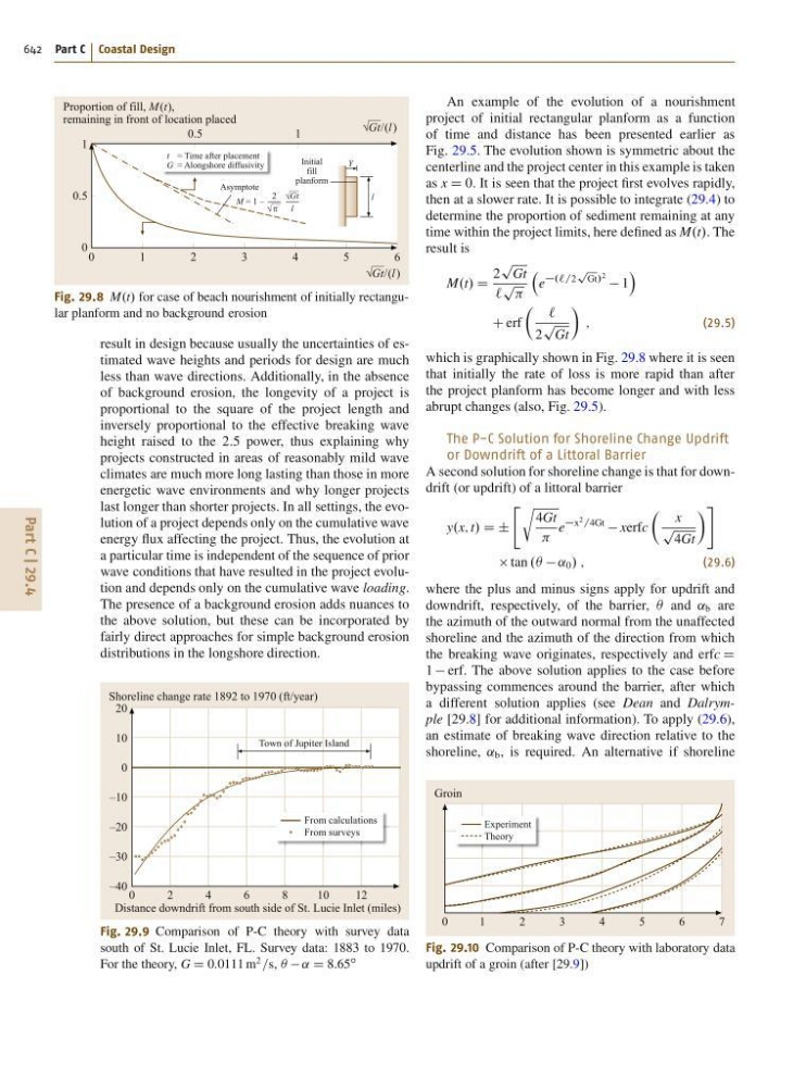
Fig. 29.8 M.t/ for case of beach nourishment of initially rectangular planform and no background erosion
result in design because usually the uncertainties of estimated wave heights and periods for design are much
less than wave directions. Additionally, in the absence
of background erosion, the longevity of a project is
proportional to the square of the project length and
inversely proportional to the effective breaking wave
height raised to the 2:5 power, thus explaining why
projects constructed in areas of reasonably mild wave
climates are much more long lasting than those in more
energetic wave environments and why longer projects
last longer than shorter projects. In all settings, the evolution of a project depends only on the cumulative wave
energy flux affecting the project. Thus, the evolution at
a particular time is independent of the sequence of prior
wave conditions that have resulted in the project evolution and depends only on the cumulative wave loading.
The presence of a background erosion adds nuances to
the above solution, but these can be incorporated by
fairly direct approaches for simple background erosion
distributions in the longshore direction.
From calculations
From surveys
0
2
4
8
Town of Jupiter Island
6
1 0
1 2
Shoreline change rate 1892 to 1970 (ft/year)
Distance downdrift from south side of St. Lucie Inlet (miles)
20
10
0
–10
–20
–30
–40
Fig. 29.9 Comparison of P-C theory with survey data
south of St. Lucie Inlet, FL. Survey data: 1883 to 1970.
For the theory, G D 0:0111 m
2
=s, Â ˛ D 8:65
ı
An example of the evolution of a nourishment
project of initial rectangular planform as a function
of time and distance has been presented earlier as
Fig. 29.5. The evolution shown is symmetric about the
centerline and the project center in this example is taken
as x D 0. It is seen that the project first evolves rapidly,
then at a slower rate. It is possible to integrate (29.4) to
determine the proportion of sediment remaining at any
time within the project limits, here defined as M.t/. The
result is
M.t/ D
2
p
Gt
`
p
e
.`=2
p
Gt/ 2 1
Á
C erf
 `
2
p
Gt
Ã
;
(29.5)
which is graphically shown in Fig. 29.8 where it is seen
that initially the rate of loss is more rapid than after
the project planform has become longer and with less
abrupt changes (also, Fig. 29.5).
The P-C Solution for Shoreline Change Updrift
or Downdrift of a Littoral Barrier
A second solution for shoreline change is that for downdrift (or updrift) of a littoral barrier
y.x; t/ D ˙
" r
4Gt
e
x 2 =4Gt
xerfc
 x
p
4Gt
à #
tan . ˛ 0 / ;
(29.6)
where the plus and minus signs apply for updrift and
downdrift, respectively, of the barrier, Â and ˛ b are
the azimuth of the outward normal from the unaffected
shoreline and the azimuth of the direction from which
the breaking wave originates, respectively and erfc D
1 erf. The above solution applies to the case before
bypassing commences around the barrier, after which
a different solution applies (see Dean and Dalrymple [29.8] for additional information). To apply (29.6),
an estimate of breaking wave direction relative to the
shoreline, ˛ b , is required. An alternative if shoreline
Experiment
Theory
0
1
2
3
4
5
6
7
Groin
Fig. 29.10 Comparison of P-C theory with laboratory data
updrift of a groin (after [29.9])