

Part C | 28.2
618 Part C Coastal Design
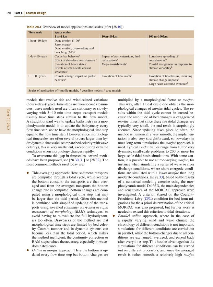
Table 28.1 Overview of model applications and scales (after [28.10])
Time scale
Space scales
1 m–1 km
10 m–10 km
100 m–100 km
1 hour–10 days
Dune erosion (1-D) a
Reset events c
Dune erosion, overwashing and
breaching (2-D) c
1 day–10 years
Cyclic bar behavior a
Effect of shoreface nourishments a
Evolution of beach states c
Effects of small-scale coastal
structures c
Impact of port extensions, land
reclamations c
Mega nourishments c
Longshore spreading of
nourishments b
Coastal realignment in response to
climate variability b
11000 years
Climate change impact on profile
behavior
a
Evolution of tidal inlets
c
Evolution of tidal basins, including
climate change impacts
c
Large-scale coastline evolution
b
Scales of application of a profile models, b coastline models, c area models
models that resolve tide and wind-related variations
(hours–days) typical time steps are from seconds to minutes; wave models used are often stationary or slowlyvarying with 510 min time steps; transport models
usually have time steps similar to the flow model.
A straightforward way to update bathymetry in a morphodynamic model is to update the bathymetry every
flow time step, and to have the morphological time step
equal to the flow time step. However, since morphological timescales are often several orders larger than hydrodynamic timescales (compare bed celerity with wave
celerity), this is very inefficient, except during extreme
conditions when morphology changes rapidly.
To overcome this gap in timescales, several methods have been proposed, see [28.30, 31] or [28.32]. The
most common methods used today are:
Tide-averaging approach: Here, sediment transports
are computed through a tidal cycle, while keeping
the bottom constant; the transports are then averaged and from the averaged transports the bottom
change rate is computed; bottom changes are computed using a morphological time step that may
be larger than the tidal period. Often this method
is combined with simplified updating of the transports using so-called continuity correction or rapid
assessment of morphology (RAM) techniques, to
avoid having to re-evaluate the full hydrodynamics too often. Drawbacks of the method are that
morphological time steps are limited by bed celerity Courant number and in dynamic systems can
become less than the tidal period, which makes
the method inefficient; the continuity correction or
RAM steps reduce the accuracy, especially in wavedominated cases.
Online or morfac approach: Here the bottom is updated every flow time step but bottom changes are
multiplied by a morphological factor or morfac.
This way, after 1 tidal cycle one obtains the morphological changes of morfac tidal cycles. The results within the tidal cycle cannot be trusted because the amplitude of bed changes is exaggerated
morfac times, but since these intratidal changes are
typically very small, the end result is surprisingly
accurate. Since updating takes place so often, the
method is numerically very smooth; the implementation is also very straightforward, so nowadays in
most long-term simulations the morfac approach is
used. Typical morfac values range from 10 for very
dynamic, small-scale problems to 200 or more for
large-scale tidal basin simulations. With some caution, it is possible to use a time-varying morfac, for
instance when simulating a series of wave or river
discharge conditions, where short energetic conditions are simulated with a lower morfac than long
moderate conditions. In [28.33], based on the results
of a numerical modeling exercise using the morphodynamic model Delft3D, the main dependencies
and sensitivities of the MORFAC approach were
investigated. A criterion (based on the Courant–
Friedrichs–Lévy (CFL) condition for bed form migration) for the a priori determination of the critical
MORFAC was also proposed, but further work is
needed to extend this criterion to tidal situations.
Parallel online approach, where in the case of
a rapidly varying wind and wave climate the
chronology of different conditions is not important,
simulations for different conditions are carried out
in parallel, while the bottom changes due to all conditions are exchanged, averaged, and passed back
after every time step. This has the advantage that the
simulations for different conditions can be carried
out on different processors, and since the averaged
result is rather smooth, a relatively high morfac