Part C | 26.3
580 Part C Coastal Design
can be used for estimating the expected width of the
confidence bands for a specified return period. The dependence of the confidence limits as a function of the
mean recurrence interval and the presence of the square
root of the sample number in the denominator show that
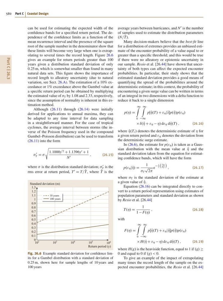
these limits will become very large when one is extrapolating to several times the record length. Figure 26.6
gives an example for return periods greater than 100
years given a distribution standard deviation of only
0:25 m, which is somewhat smaller than found in many
natural data sets. This figure shows the importance of
record length to alleatory uncertainty (due to natural
variation, see Sect. 26.A). The estimation of a 10% exceedance or 1% exceedance above the Gumbel value at
a specific return period can be obtained by multiplying
the estimated value of T by 1.08 and 2.33, respectively,
since the assumption of normality is inherent in this estimation method.
Although (26.11) through (26.14) were initially
derived for applications to annual maxima, they can
be adapted to any time interval for data sampling
in a straightforward manner. For the case of tropical
cyclones, the average interval between storms (the inverse of the Poisson frequency used in the compound
Gumbel–Poisson distribution) can be used to transform
(26.11) into the form
0
T D
s
1:1000y
0 2 C 1:1396y 0 C 1
N 0
;
(26.15)
where is the distribution standard deviation;
0
T is the
rms error at return period, T
0
D T= O
T, where O
T is the
10 years
100 years
10
2
10
3
10
4
10
5
10
6
Standard deviation (m)
Return period (y)
1.3
1.2
1.1
1
0.9
0.8
0.7
0.6
0.5
0.4
0.3
0.2
0.1
0
Fig. 26.6 Example standard deviation for confidence limits for a Gumbel distribution with a standard deviation of
0:25 m, shown here for sample lengths of 10 years and
100 years
average years between hurricanes, and N
0 is the number
of samples used to estimate the distribution parameters
.N= O
T/.
Many decision-makers believe that the best-fit line
for a distribution of extremes provides an unbiased estimate of the encounter probability of a value equal to or
greater than a specific threshold; and this would be true
if there were no alleatory or epistemic uncertainty in
our sample. Resio et al. [26.44] have shown that uncertainty of both types can affect the expected encounter
probabilities. In particular, their study shows that the
estimated standard deviation provides a good means of
quantifying the spread of the probabilities around the
deterministic estimate; in this context, the probability of
encountering a given surge value can be written in terms
of an integral in two dimensions with a delta function to
reduce it back to a single dimension
p.Á/ D
1
Z
0
1
Z
1
pΠO
Á.T/ C " Á jO xp. O
Á/p." Á /
ı. O
Á C " Á Á/ d" Á d O
Á.T/ ;
(26.16)
where O
Á.T r / denotes the deterministic estimate of Á for
a given return period and " Á denotes the deviation from
the deterministic surge estimate.
In (26.6), the estimate for p." Á / is taken as a Gaussian distribution with the mean value at O
Á and the
standard deviation taken from the equation for estimating confidence bands, which will have the form
p." Á j O
Á/ D
1
T
p
2
e
1
2
"Á
T
Á
;
(26.17)
where T is the standard deviation of the estimate at
a given value of O
Á.
Equation (26.16) can be integrated directly to convert to a return period representation using estimates of
population parameters and standard deviation as shown
by Resio et al. [26.44]
T.Á/ D
1
1 F.Á/
;
(26.18)
with
F.Á/ D
1
Z
0
1
Z
1
pΠO
Á.T/ C " Á j O
Áp. O
Á/p." Á /
H. O
Á C " Á Á/ d" Á d O
Á.T/ ;
(26.19)
where H.g/ is the heaviside function, equal to 1 if .g/
0 and equal to 0 if .g/ < 0.
To give an example of the impact of extrapolating
many times the record length of the sample on the expected encounter probabilities, the Resio et al. [26.44]