

Statistical Characterization of Hazards and Risk in Coastal Areas 26.2 Quantifying Coastal Hazards/Risks 573
Part C | 26.2
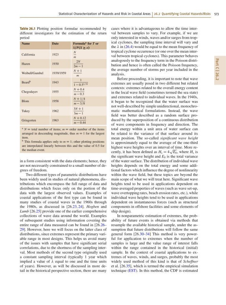
Table 26.1 Plotting position formulae recommended by
different investigators for the estimation of the return
period
Name
Date
Formula a for T or
1=P.X x/
California
1923
N
m
Hazen
1930
2N
2m 1
Weibull/Gumbel
1939/1959
N C 1
m
Beard b
1943
1
1 0:5 1=N
Chegodayev
1955
N C 0:4
m 0:3
Blom
1958
N C 1=4
m 3=8
Tukey
1962
3N C 1
3m 1
Gringorten
1963
N C 0:12
m 0:44
a N D total number of items; m D order number of the items
arranged in descending magnitude, thus m D 1 for the largest
item.
b This formula applies only to m D 1; other plotting positions
are interpolated linearly between this and the value of 0.5 for
the median event.
in a form consistent with the data elements; hence, they
are not necessarily constrained to a small number of degrees of freedom.
Two different types of parametric distributions have
been widely used in studies of natural phenomena, distributions which encompass the full range of data and
distributions which focus only on the portion of the
data with the largest observed values. Examples of
coastal applications of the first type can be found in
many studies of coastal waves in the 1960s through
the 1980s, as discussed in [26.23, 24]. Hogben and
Lumb [26.25] provide one of the earlier comprehensive
collections of wave data around the world. Examples
of subsequent studies using information covering the
entire range of data measured can be found in [26.26–
29]. However, here we will focus on the latter class of
distributions, since extremes represent the primary variable range in most designs. This helps us avoid many
of the issues with samples that have significant serial
correlations, due to the shortness of the sampling interval. Most methods of the second type originally used
a constant sampling interval (typically 1 year which
implied a value of equal to one and the time units
of years). However, as will be discussed in more detail in the historical perspective section, there are many
cases where it is advantageous to allow the time interval between samples to vary. For example, if we are
only interested in winds, waves and/or surges from tropical cyclones, the sampling time interval will vary and
the in (26.4) would be equal to the mean frequency of
tropical cyclone occurrence (or one over the mean interval between tropical cyclones). This parameter behaves
analogously to the frequency term in the Poisson distribution and hence is often called the Poisson frequency,
the average number of storms per year included in the
analysis.
Before proceeding, it is important to note that wave
extremes are usually posed in two different but related
contexts: extremes related to the overall energy content
in the local wave field (sometimes termed the sea state)
and extremes related to individual waves. In the 1940s,
it began to be recognized that the water surface was
not well-described by simple unidirectional, monochromatic mathematical formulations. Instead, the wave
field was better described as a random surface produced by the superposition of a continuous distribution
of wave components in frequency and direction. The
total energy within a unit area of water surface can
be related to the variance of that surface around its
mean position. The so-called significant wave height
is approximately equal to the average of the one-third
highest wave heights over an interval of time. More recently, it has been defined as H s D 4
p
E 0 , where H s is
the significant wave height and E 0 is the total variance
of the water surface. The distribution of individual wave
heights depends on the total energy and some additional factors which influence the degree of nonlinearity
within the wave field, but these topics are beyond the
main scope of what we will treat here. Significant wave
heights tend to be used in applications dependent on
time-averaged properties of waves (such as wave set-up,
wave overtopping rates, beach erosion rates, etc.), while
individual wave heights tend to be used in applications
dependent on instantaneous forces (such as structural
components in offshore facilities and some elements of
ship design).
In nonparametric estimation of extremes, the probability of future events is obtained via methods that
resample the available historical sample, under the assumption that future distributions will follow the same
general form [26.30–34] This method is very powerful for application to extremes when the number of
samples is large and the value range of interest falls
within the range contained in the historical (initial)
sample. In the context of coastal applications to extremes of waves, winds, and surges, probably the most
widely used method of this kind is that of Scheffner
et al. [26.35], which is termed the empirical simulation
technique (EST). In this method, the CDF is estimated