

Part C | 26.2
572 Part C Coastal Design
0
50
100
150
200
250
Probability of exceeding 100-year value
Years duration
1
0.8
0.6
0.4
0.2
0
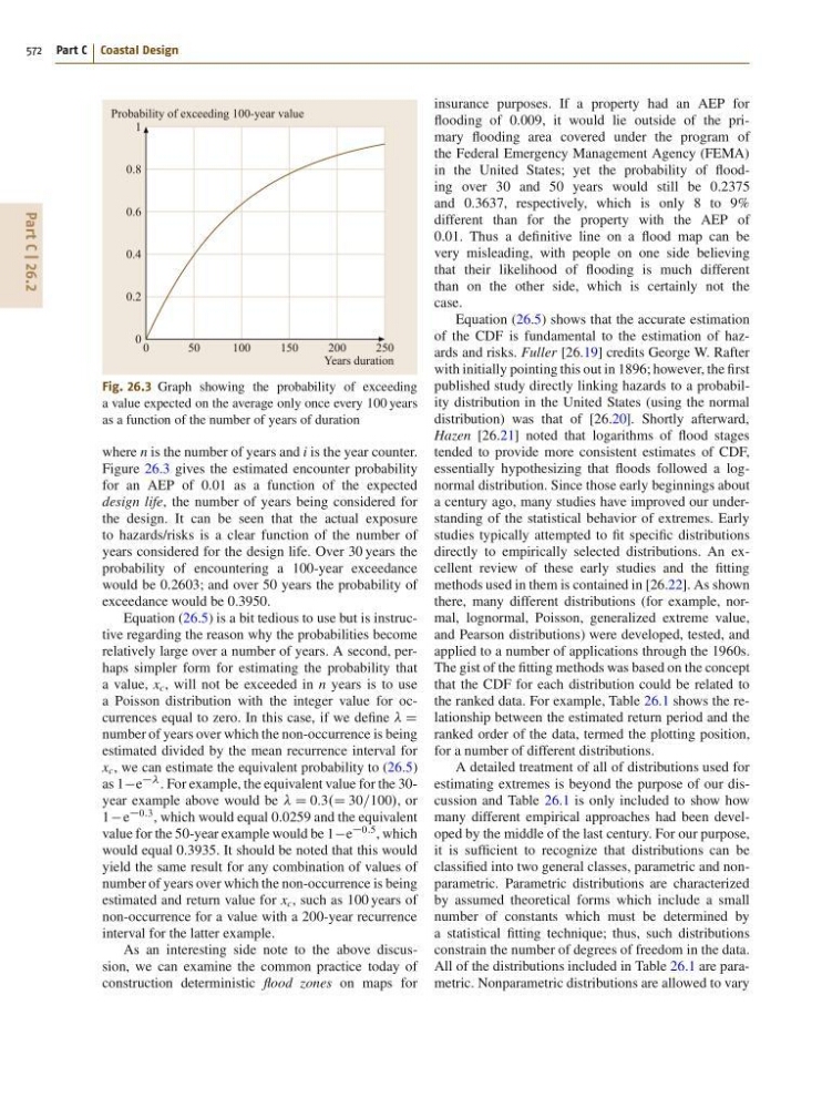
Fig. 26.3 Graph showing the probability of exceeding
a value expected on the average only once every 100 years
as a function of the number of years of duration
where n is the number of years and i is the year counter.
Figure 26.3 gives the estimated encounter probability
for an AEP of 0.01 as a function of the expected
design life, the number of years being considered for
the design. It can be seen that the actual exposure
to hazards/risks is a clear function of the number of
years considered for the design life. Over 30 years the
probability of encountering a 100-year exceedance
would be 0.2603; and over 50 years the probability of
exceedance would be 0.3950.
Equation (26.5) is a bit tedious to use but is instructive regarding the reason why the probabilities become
relatively large over a number of years. A second, perhaps simpler form for estimating the probability that
a value, x c , will not be exceeded in n years is to use
a Poisson distribution with the integer value for occurrences equal to zero. In this case, if we define D
number of years over which the non-occurrence is being
estimated divided by the mean recurrence interval for
x c , we can estimate the equivalent probability to (26.5)
as 1e
. For example, the equivalent value for the 30year example above would be D 0:3.D 30=100/, or
1 e
0:3 , which would equal 0.0259 and the equivalent
value for the 50-year example would be 1e
0:5 , which
would equal 0.3935. It should be noted that this would
yield the same result for any combination of values of
number of years over which the non-occurrence is being
estimated and return value for x c , such as 100 years of
non-occurrence for a value with a 200-year recurrence
interval for the latter example.
As an interesting side note to the above discussion, we can examine the common practice today of
construction deterministic flood zones on maps for
insurance purposes. If a property had an AEP for
flooding of 0.009, it would lie outside of the primary flooding area covered under the program of
the Federal Emergency Management Agency (FEMA)
in the United States; yet the probability of flooding over 30 and 50 years would still be 0.2375
and 0.3637, respectively, which is only 8 to 9%
different than for the property with the AEP of
0.01. Thus a definitive line on a flood map can be
very misleading, with people on one side believing
that their likelihood of flooding is much different
than on the other side, which is certainly not the
case.
Equation (26.5) shows that the accurate estimation
of the CDF is fundamental to the estimation of hazards and risks. Fuller [26.19] credits George W. Rafter
with initially pointing this out in 1896; however, the first
published study directly linking hazards to a probability distribution in the United States (using the normal
distribution) was that of [26.20]. Shortly afterward,
Hazen [26.21] noted that logarithms of flood stages
tended to provide more consistent estimates of CDF,
essentially hypothesizing that floods followed a lognormal distribution. Since those early beginnings about
a century ago, many studies have improved our understanding of the statistical behavior of extremes. Early
studies typically attempted to fit specific distributions
directly to empirically selected distributions. An excellent review of these early studies and the fitting
methods used in them is contained in [26.22]. As shown
there, many different distributions (for example, normal, lognormal, Poisson, generalized extreme value,
and Pearson distributions) were developed, tested, and
applied to a number of applications through the 1960s.
The gist of the fitting methods was based on the concept
that the CDF for each distribution could be related to
the ranked data. For example, Table 26.1 shows the relationship between the estimated return period and the
ranked order of the data, termed the plotting position,
for a number of different distributions.
A detailed treatment of all of distributions used for
estimating extremes is beyond the purpose of our discussion and Table 26.1 is only included to show how
many different empirical approaches had been developed by the middle of the last century. For our purpose,
it is sufficient to recognize that distributions can be
classified into two general classes, parametric and nonparametric. Parametric distributions are characterized
by assumed theoretical forms which include a small
number of constants which must be determined by
a statistical fitting technique; thus, such distributions
constrain the number of degrees of freedom in the data.
All of the distributions included in Table 26.1 are parametric. Nonparametric distributions are allowed to vary