

Part B | 14.2
350 Part B Autonomous Ocean Vehicles, Subsystems and Control
reliability of any of these approaches will depend on the
accuracy of the a priori map.
AUV navigation based on bathymetric data has
been successfully achieved by Bergem [14.66]. In this
system, depths are measured at different angles using
a multibeam sonar. This gives an accurate profile of the
sea floor, and the absolute position is determined by
matching this profile against an a priori known detailed
bathymetric map of the actual area. This idea is motivated by the successful employment of this technique
to missile guidance systems.
14.2.4 Simultaneous Localization
and Mapping
In practice, an up-to-date, high-quality map may be
unavailable in the operating area of interest. This motivates research into the use of SLAM to enable an
AUV to build a map of its environment while concurrently using that map to navigate in real time [14.67].
SLAM is a probabilistic estimation problem in which
noisy sensor measurements are combined into a probabilistic representation of the state of the sensor and the
observed surroundings. This model needs to be updated
and extended sequentially by integrating new sensor
measurements as they become available.
The variables to be estimated and the sensor measurements can be described in a graph [14.68] that
captures their relation. We use a factor graph [14.69]
as a general graphical model representation of the
SLAM problem. Formally, a factor graph is a bipartite
graph G D .F; ;; E/ with two node types: factor nodes
f i 2 F and variable nodes  j 2 . Edges e ij 2 E are always between factor nodes and variable nodes. A factor
graph G defines the factorization of a function f ../ as
f ../ D
Y
i
f i .. i / ;
(14.3)
where i is the set of variables  j adjacent to the factor f i , and independent relationships are encoded by the
edges e ij : each factor f i is a function of the variables in
i . Our goal is to find the variable assignment
that
maximizes (14.3)
D arg max
f ../ :
(14.4)
The general factor graph formulation of the full
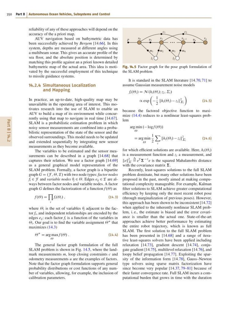
SLAM problem is shown in Fig. 14.5, where the landmark measurements m, loop closing constraints c and
odometry measurements u are the examples of factors.
Note that the factor graph formulation supports general
probability distributions or cost functions of any number of variables, allowing, for example, the inclusion of
calibration parameters.
l 1
l 2
u 1
x 1
x 0
u n
x n
x n –1
p
m 2
m 1
m 4
c 2
c 1
m 3
Fig. 14.5 Factor graph for the pose graph formulation of
the SLAM problem
It is standard in the SLAM literature [14.70, 71] to
assume Gaussian measurement noise models
f i .. i / D N .h i .. i /I z i ; ˙ i /
/ exp
Â
1
2
kh i .. i / z i k
2
˙i
Ã
(14.5)
because the factored objective function to maximize (14.4) reduces to a nonlinear least-squares problem
arg min
. log f ..//
D arg min
1
2
X
i
kh i .. i / z i k
2
˙i
(14.6)
for which efficient solutions are available. Here, h i .. i /
is a measurement function and z i a measurement, and
kek
2
˙
D e
T
†
1 e is the squared Mahalanobis distance
with the covariance matrix †.
Recently, least-squares solutions to the full SLAM
problem dominate, but many other solutions have been
proposed in the past, mostly aimed at making computational complexity manageable. For example, Kalman
filter solutions to SLAM achieve greater computational
efficiency by keeping only the most recent robot pose
(through marginalization of previous poses). However,
this approach has been shown to be inconsistent [14.72]
when applied to the inherently nonlinear SLAM problem, i. e., the estimate is biased and the error covariance is smaller than the actual one. State-of-the-art
approaches achieve better performance by estimating
the entire robot trajectory, which is known as full
SLAM. The first solution to the full SLAM problem
has been presented in [14.68] and a range of iterative least-squares solvers have been applied including
relaxation [14.73], gradient descent [14.74], conjugate gradient [14.75], multilevel relaxation [14.76], and
loopy belief propagation [14.77]. Exploiting the sparsity of the information form [14.78], Gauss–Newton
type solvers using sparse matrix factorization have
since become very popular [14.37, 79–81] because of
their faster convergence rate. Full SLAM incurs a computational burden that grows in time with the duration
350 Part B Autonomous Ocean Vehicles, Subsystems and Control
reliability of any of these approaches will depend on the
accuracy of the a priori map.
AUV navigation based on bathymetric data has
been successfully achieved by Bergem [14.66]. In this
system, depths are measured at different angles using
a multibeam sonar. This gives an accurate profile of the
sea floor, and the absolute position is determined by
matching this profile against an a priori known detailed
bathymetric map of the actual area. This idea is motivated by the successful employment of this technique
to missile guidance systems.
14.2.4 Simultaneous Localization
and Mapping
In practice, an up-to-date, high-quality map may be
unavailable in the operating area of interest. This motivates research into the use of SLAM to enable an
AUV to build a map of its environment while concurrently using that map to navigate in real time [14.67].
SLAM is a probabilistic estimation problem in which
noisy sensor measurements are combined into a probabilistic representation of the state of the sensor and the
observed surroundings. This model needs to be updated
and extended sequentially by integrating new sensor
measurements as they become available.
The variables to be estimated and the sensor measurements can be described in a graph [14.68] that
captures their relation. We use a factor graph [14.69]
as a general graphical model representation of the
SLAM problem. Formally, a factor graph is a bipartite
graph G D .F; ;; E/ with two node types: factor nodes
f i 2 F and variable nodes  j 2 . Edges e ij 2 E are always between factor nodes and variable nodes. A factor
graph G defines the factorization of a function f ../ as
f ../ D
Y
i
f i .. i / ;
(14.3)
where i is the set of variables  j adjacent to the factor f i , and independent relationships are encoded by the
edges e ij : each factor f i is a function of the variables in
i . Our goal is to find the variable assignment
that
maximizes (14.3)
D arg max
f ../ :
(14.4)
The general factor graph formulation of the full
SLAM problem is shown in Fig. 14.5, where the landmark measurements m, loop closing constraints c and
odometry measurements u are the examples of factors.
Note that the factor graph formulation supports general
probability distributions or cost functions of any number of variables, allowing, for example, the inclusion of
calibration parameters.
l 1
l 2
u 1
x 1
x 0
u n
x n
x n –1
p
m 2
m 1
m 4
c 2
c 1
m 3
Fig. 14.5 Factor graph for the pose graph formulation of
the SLAM problem
It is standard in the SLAM literature [14.70, 71] to
assume Gaussian measurement noise models
f i .. i / D N .h i .. i /I z i ; ˙ i /
/ exp
Â
1
2
kh i .. i / z i k
2
˙i
Ã
(14.5)
because the factored objective function to maximize (14.4) reduces to a nonlinear least-squares problem
arg min
. log f ..//
D arg min
1
2
X
i
kh i .. i / z i k
2
˙i
(14.6)
for which efficient solutions are available. Here, h i .. i /
is a measurement function and z i a measurement, and
kek
2
˙
D e
T
†
1 e is the squared Mahalanobis distance
with the covariance matrix †.
Recently, least-squares solutions to the full SLAM
problem dominate, but many other solutions have been
proposed in the past, mostly aimed at making computational complexity manageable. For example, Kalman
filter solutions to SLAM achieve greater computational
efficiency by keeping only the most recent robot pose
(through marginalization of previous poses). However,
this approach has been shown to be inconsistent [14.72]
when applied to the inherently nonlinear SLAM problem, i. e., the estimate is biased and the error covariance is smaller than the actual one. State-of-the-art
approaches achieve better performance by estimating
the entire robot trajectory, which is known as full
SLAM. The first solution to the full SLAM problem
has been presented in [14.68] and a range of iterative least-squares solvers have been applied including
relaxation [14.73], gradient descent [14.74], conjugate gradient [14.75], multilevel relaxation [14.76], and
loopy belief propagation [14.77]. Exploiting the sparsity of the information form [14.78], Gauss–Newton
type solvers using sparse matrix factorization have
since become very popular [14.37, 79–81] because of
their faster convergence rate. Full SLAM incurs a computational burden that grows in time with the duration