

Part B | 14.2
346 Part B Autonomous Ocean Vehicles, Subsystems and Control
Beacon 1
Beacon 2
Beacon 3
Beacon 4
0
100
200
300
400
500
600
700
800
Travel time (s)
Mission time (s)
2
1.8
1.6
1.4
1.2
1
0.8
0.6
0.4
0.2
0
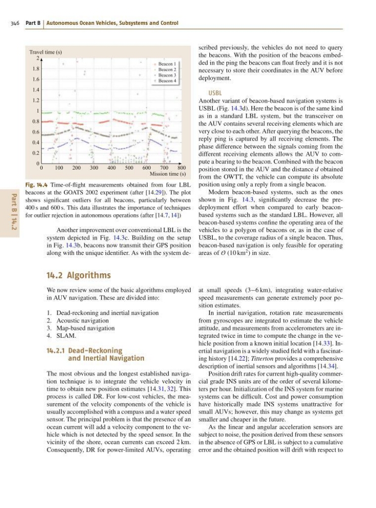
Fig. 14.4 Time-of-flight measurements obtained from four LBL
beacons at the GOATS 2002 experiment (after [14.29]). The plot
shows significant outliers for all beacons, particularly between
400 s and 600 s. This data illustrates the importance of techniques
for outlier rejection in autonomous operations (after [14.7, 14])
Another improvement over conventional LBL is the
system depicted in Fig. 14.3c. Building on the setup
in Fig. 14.3b, beacons now transmit their GPS position
along with the unique identifier. As with the system described previously, the vehicles do not need to query
the beacons. With the position of the beacons embedded in the ping the beacons can float freely and it is not
necessary to store their coordinates in the AUV before
deployment.
USBL
Another variant of beacon-based navigation systems is
USBL (Fig. 14.3d). Here the beacon is of the same kind
as in a standard LBL system, but the transceiver on
the AUV contains several receiving elements which are
very close to each other. After querying the beacons, the
reply ping is captured by all receiving elements. The
phase difference between the signals coming from the
different receiving elements allows the AUV to compute a bearing to the beacon. Combined with the beacon
position stored in the AUV and the distance d obtained
from the OWTT, the vehicle can compute its absolute
position using only a reply from a single beacon.
Modern beacon-based systems, such as the ones
shown in Fig. 14.3, significantly decrease the predeployment effort when compared to early beaconbased systems such as the standard LBL. However, all
beacon-based systems confine the operating area of the
vehicles to a polygon of beacons or, as in the case of
USBL, to the coverage radius of a single beacon. Thus,
beacon-based navigation is only feasible for operating
areas of O (10 km
2 ) in size.
14.2 Algorithms
We now review some of the basic algorithms employed
in AUV navigation. These are divided into:
1. Dead-reckoning and inertial navigation
2. Acoustic navigation
3. Map-based navigation
4. SLAM.
14.2.1 Dead-Reckoning
and Inertial Navigation
The most obvious and the longest established navigation technique is to integrate the vehicle velocity in
time to obtain new position estimates [14.31, 32]. This
process is called DR. For low-cost vehicles, the measurement of the velocity components of the vehicle is
usually accomplished with a compass and a water speed
sensor. The principal problem is that the presence of an
ocean current will add a velocity component to the vehicle which is not detected by the speed sensor. In the
vicinity of the shore, ocean currents can exceed 2 km.
Consequently, DR for power-limited AUVs, operating
at small speeds (36 km), integrating water-relative
speed measurements can generate extremely poor position estimates.
In inertial navigation, rotation rate measurements
from gyroscopes are integrated to estimate the vehicle
attitude, and measurements from accelerometers are integrated twice in time to compute the change in the vehicle position from a known initial location [14.33]. Inertial navigation is a widely studied field with a fascinating history [14.22]; Titterton provides a comprehensive
description of inertial sensors and algorithms [14.34].
Position drift rates for current high-quality commercial grade INS units are of the order of several kilometers per hour. Initialization of the INS system for marine
systems can be difficult. Cost and power consumption
have historically made INS systems unattractive for
small AUVs; however, this may change as systems get
smaller and cheaper in the future.
As the linear and angular acceleration sensors are
subject to noise, the position derived from these sensors
in the absence of GPS or LBL is subject to a cumulative
error and the obtained position will drift with respect to
346 Part B Autonomous Ocean Vehicles, Subsystems and Control
Beacon 1
Beacon 2
Beacon 3
Beacon 4
0
100
200
300
400
500
600
700
800
Travel time (s)
Mission time (s)
2
1.8
1.6
1.4
1.2
1
0.8
0.6
0.4
0.2
0
Fig. 14.4 Time-of-flight measurements obtained from four LBL
beacons at the GOATS 2002 experiment (after [14.29]). The plot
shows significant outliers for all beacons, particularly between
400 s and 600 s. This data illustrates the importance of techniques
for outlier rejection in autonomous operations (after [14.7, 14])
Another improvement over conventional LBL is the
system depicted in Fig. 14.3c. Building on the setup
in Fig. 14.3b, beacons now transmit their GPS position
along with the unique identifier. As with the system described previously, the vehicles do not need to query
the beacons. With the position of the beacons embedded in the ping the beacons can float freely and it is not
necessary to store their coordinates in the AUV before
deployment.
USBL
Another variant of beacon-based navigation systems is
USBL (Fig. 14.3d). Here the beacon is of the same kind
as in a standard LBL system, but the transceiver on
the AUV contains several receiving elements which are
very close to each other. After querying the beacons, the
reply ping is captured by all receiving elements. The
phase difference between the signals coming from the
different receiving elements allows the AUV to compute a bearing to the beacon. Combined with the beacon
position stored in the AUV and the distance d obtained
from the OWTT, the vehicle can compute its absolute
position using only a reply from a single beacon.
Modern beacon-based systems, such as the ones
shown in Fig. 14.3, significantly decrease the predeployment effort when compared to early beaconbased systems such as the standard LBL. However, all
beacon-based systems confine the operating area of the
vehicles to a polygon of beacons or, as in the case of
USBL, to the coverage radius of a single beacon. Thus,
beacon-based navigation is only feasible for operating
areas of O (10 km
2 ) in size.
14.2 Algorithms
We now review some of the basic algorithms employed
in AUV navigation. These are divided into:
1. Dead-reckoning and inertial navigation
2. Acoustic navigation
3. Map-based navigation
4. SLAM.
14.2.1 Dead-Reckoning
and Inertial Navigation
The most obvious and the longest established navigation technique is to integrate the vehicle velocity in
time to obtain new position estimates [14.31, 32]. This
process is called DR. For low-cost vehicles, the measurement of the velocity components of the vehicle is
usually accomplished with a compass and a water speed
sensor. The principal problem is that the presence of an
ocean current will add a velocity component to the vehicle which is not detected by the speed sensor. In the
vicinity of the shore, ocean currents can exceed 2 km.
Consequently, DR for power-limited AUVs, operating
at small speeds (36 km), integrating water-relative
speed measurements can generate extremely poor position estimates.
In inertial navigation, rotation rate measurements
from gyroscopes are integrated to estimate the vehicle
attitude, and measurements from accelerometers are integrated twice in time to compute the change in the vehicle position from a known initial location [14.33]. Inertial navigation is a widely studied field with a fascinating history [14.22]; Titterton provides a comprehensive
description of inertial sensors and algorithms [14.34].
Position drift rates for current high-quality commercial grade INS units are of the order of several kilometers per hour. Initialization of the INS system for marine
systems can be difficult. Cost and power consumption
have historically made INS systems unattractive for
small AUVs; however, this may change as systems get
smaller and cheaper in the future.
As the linear and angular acceleration sensors are
subject to noise, the position derived from these sensors
in the absence of GPS or LBL is subject to a cumulative
error and the obtained position will drift with respect to