

Control Theory and Applications 10.3 SISO System Controls 257
Part A | 10.3
–
+
Y d (s)
Y (s)
E (s)
A/D
Σ
D/A
H (s)
PC
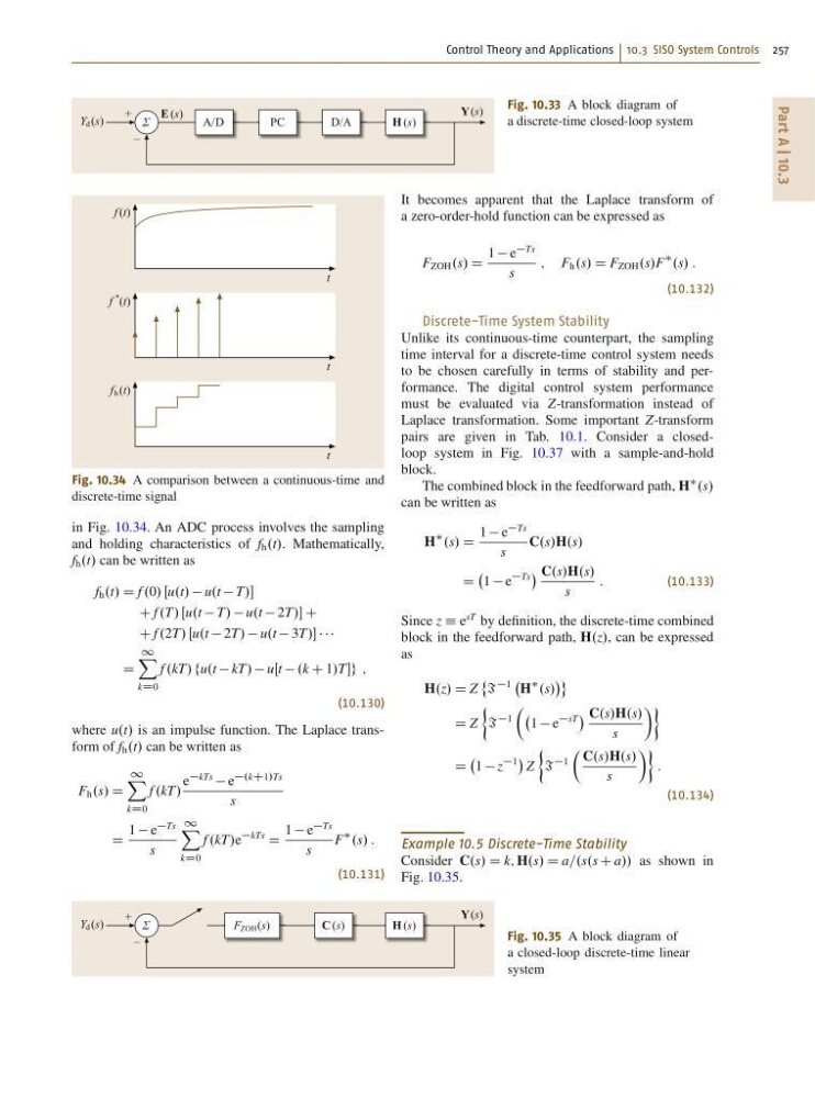
Fig. 10.33 A block diagram of
a discrete-time closed-loop system
t
f (t)
t
f
* (t)
t
f h (t)
Fig. 10.34 A comparison between a continuous-time and
discrete-time signal
in Fig. 10.34. An ADC process involves the sampling
and holding characteristics of f h .t/. Mathematically,
f h .t/ can be written as
f h .t/ D f .0/ Œu.t/ u.t T/
C f .T/ Œu.t T/ u.t 2T/ C
C f .2T/ Œu.t 2T/ u.t 3T/
D
1
X
kD0
f .kT/ fu.t kT/ uŒt .k C 1/Tg ;
(10.130)
where u.t/ is an impulse function. The Laplace transform of f h .t/ can be written as
F h .s/ D
1
X
kD0
f .kT/
e
kTs
e
.kC1/Ts
s
D
1 e
Ts
s
1
X
kD0
f .kT/e
kTs
D
1 e
Ts
s
F
.s/ :
(10.131)
–
+
Y d (s)
Y (s)
F ZOH (s)
Σ
C (s)
H (s)
Fig. 10.35 A block diagram of
a closed-loop discrete-time linear
system
It becomes apparent that the Laplace transform of
a zero-order-hold function can be expressed as
F ZOH .s/ D
1 e
Ts
s
; F h .s/ D F ZOH .s/F
.s/ :
(10.132)
Discrete-Time System Stability
Unlike its continuous-time counterpart, the sampling
time interval for a discrete-time control system needs
to be chosen carefully in terms of stability and performance. The digital control system performance
must be evaluated via Z-transformation instead of
Laplace transformation. Some important Z-transform
pairs are given in Tab. 10.1. Consider a closedloop system in Fig. 10.37 with a sample-and-hold
block.
The combined block in the feedforward path, H
.s/
can be written as
H
.s/ D
1 e
Ts
s
C.s/H.s/
D
1 e
Ts
C.s/H.s/
s
:
(10.133)
Since z Á e
sT by definition, the discrete-time combined
block in the feedforward path, H.z/, can be expressed
as
H.z/ D Z
˚ I
1
H
.s/
«
D Z
I
1
Â
1 e
sT
C.s/H.s/
s
ÃÃ
D
1 z
1
Z
I
1
 C.s/H.s/
s
ÃÃ
:
(10.134)
Example 10.5 Discrete-Time Stability
Consider C.s/ D k; H.s/ D a=.s.s C a// as shown in
Fig. 10.35.
Part A | 10.3
–
+
Y d (s)
Y (s)
E (s)
A/D
Σ
D/A
H (s)
PC
Fig. 10.33 A block diagram of
a discrete-time closed-loop system
t
f (t)
t
f
* (t)
t
f h (t)
Fig. 10.34 A comparison between a continuous-time and
discrete-time signal
in Fig. 10.34. An ADC process involves the sampling
and holding characteristics of f h .t/. Mathematically,
f h .t/ can be written as
f h .t/ D f .0/ Œu.t/ u.t T/
C f .T/ Œu.t T/ u.t 2T/ C
C f .2T/ Œu.t 2T/ u.t 3T/
D
1
X
kD0
f .kT/ fu.t kT/ uŒt .k C 1/Tg ;
(10.130)
where u.t/ is an impulse function. The Laplace transform of f h .t/ can be written as
F h .s/ D
1
X
kD0
f .kT/
e
kTs
e
.kC1/Ts
s
D
1 e
Ts
s
1
X
kD0
f .kT/e
kTs
D
1 e
Ts
s
F
.s/ :
(10.131)
–
+
Y d (s)
Y (s)
F ZOH (s)
Σ
C (s)
H (s)
Fig. 10.35 A block diagram of
a closed-loop discrete-time linear
system
It becomes apparent that the Laplace transform of
a zero-order-hold function can be expressed as
F ZOH .s/ D
1 e
Ts
s
; F h .s/ D F ZOH .s/F
.s/ :
(10.132)
Discrete-Time System Stability
Unlike its continuous-time counterpart, the sampling
time interval for a discrete-time control system needs
to be chosen carefully in terms of stability and performance. The digital control system performance
must be evaluated via Z-transformation instead of
Laplace transformation. Some important Z-transform
pairs are given in Tab. 10.1. Consider a closedloop system in Fig. 10.37 with a sample-and-hold
block.
The combined block in the feedforward path, H
.s/
can be written as
H
.s/ D
1 e
Ts
s
C.s/H.s/
D
1 e
Ts
C.s/H.s/
s
:
(10.133)
Since z Á e
sT by definition, the discrete-time combined
block in the feedforward path, H.z/, can be expressed
as
H.z/ D Z
˚ I
1
H
.s/
«
D Z
I
1
Â
1 e
sT
C.s/H.s/
s
ÃÃ
D
1 z
1
Z
I
1
 C.s/H.s/
s
ÃÃ
:
(10.134)
Example 10.5 Discrete-Time Stability
Consider C.s/ D k; H.s/ D a=.s.s C a// as shown in
Fig. 10.35.