

Part A | 10.3
256 Part A Fundamentals
Desired
Actual
0
5
10
15
20
25
α = 0, u lim = 1
30
35
40
45
50
Output
Time (s)
2
1.5
1
0.5
0
–0.5
–1
–1.5
–2
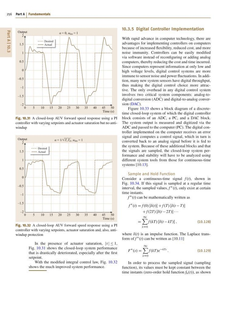
Fig. 10.31 A closed-loop AUV forward speed response using a PI
controller with varying setpoints and actuator saturation but no antiwindup
Desired
Actual
0
5
10
15
20
25
α = 1/√
—— , u lim = 1
30
35
40
45
50
Output
Time (s)
2
1.5
1
0.5
0
–0.5
–1
–1.5
–2
T i T d
Fig. 10.32 A closed-loop AUV forward speed response using a PI
controller with varying setpoints, actuator saturation and, also, antiwindup protection
In the presence of actuator saturation, jj Ä 1,
Fig. 10.31 shows the closed-loop system performance
that is drastically deteriorated, especially after the first
setpoint.
With the modified integral control law, Fig. 10.32
shows the much improved system performance.
10.3.5 Digital Controller Implementation
With rapid advance in computer technology, there are
advantages for implementing controllers on computers
because of increased flexibility, reduced cost, and more
noise immunity. Controllers can be easily modified
via software instead of reconfiguring or adding analog
computers, thereby reducing the cost and time incurred.
Since computers represent information at only low and
high voltage levels, digital control systems are more
immune to sensor noise and power fluctuations. In addition, many new system sensors have digital throughput,
thus making the digital control choice more attractive. The only overhead in any digital control system
involves two critical system components: analog-todigital conversion (ADC) and digital-to-analog conversion (DAC).
Figure 10.33 shows a block diagram of a discretetime closed-loop system of which the digital controller
block consists of an ADC, a PC, and a DAC block.
The system output is measured and digitized via the
ADC and passed to the computer (PC). The digital controller implemented on the computer receives an error
signal and computes a control signal, which in turn is
converted back to an analog signal before it is fed to
the system. Because of these additional blocks and that
the signals are sampled, the closed-loop system performance and stability will have to be analyzed using
different system tools from those for continuous-time
systems [10.13].
Sample and Hold Function
Consider a continuous-time signal f .t/, shown in
Fig. 10.34. If this signal is sampled at a regular time
interval, the sampled values, f
.t/, only exist at certain
time instants.
f
.t/ can be mathematically written as
f
.t/ D f .0/ Œı.t/ C f .T/ Œı.t T/
C f .2T/ Œı.t 2T/
D
1
X
kD0
f .kT/ Œı.t kT/ ;
(10.128)
where ı.t/ is an impulse function. The Laplace transform of f
.t/ can be written as [10.11]
F
.s/ D
1
X
kD0
f .kT/e
kTs
:
(10.129)
In order to process the sampled signal (sampling
function), its values must be kept constant between the
time instants (zero-order hold function f h .t//, as shown
256 Part A Fundamentals
Desired
Actual
0
5
10
15
20
25
α = 0, u lim = 1
30
35
40
45
50
Output
Time (s)
2
1.5
1
0.5
0
–0.5
–1
–1.5
–2
Fig. 10.31 A closed-loop AUV forward speed response using a PI
controller with varying setpoints and actuator saturation but no antiwindup
Desired
Actual
0
5
10
15
20
25
α = 1/√
—— , u lim = 1
30
35
40
45
50
Output
Time (s)
2
1.5
1
0.5
0
–0.5
–1
–1.5
–2
T i T d
Fig. 10.32 A closed-loop AUV forward speed response using a PI
controller with varying setpoints, actuator saturation and, also, antiwindup protection
In the presence of actuator saturation, jj Ä 1,
Fig. 10.31 shows the closed-loop system performance
that is drastically deteriorated, especially after the first
setpoint.
With the modified integral control law, Fig. 10.32
shows the much improved system performance.
10.3.5 Digital Controller Implementation
With rapid advance in computer technology, there are
advantages for implementing controllers on computers
because of increased flexibility, reduced cost, and more
noise immunity. Controllers can be easily modified
via software instead of reconfiguring or adding analog
computers, thereby reducing the cost and time incurred.
Since computers represent information at only low and
high voltage levels, digital control systems are more
immune to sensor noise and power fluctuations. In addition, many new system sensors have digital throughput,
thus making the digital control choice more attractive. The only overhead in any digital control system
involves two critical system components: analog-todigital conversion (ADC) and digital-to-analog conversion (DAC).
Figure 10.33 shows a block diagram of a discretetime closed-loop system of which the digital controller
block consists of an ADC, a PC, and a DAC block.
The system output is measured and digitized via the
ADC and passed to the computer (PC). The digital controller implemented on the computer receives an error
signal and computes a control signal, which in turn is
converted back to an analog signal before it is fed to
the system. Because of these additional blocks and that
the signals are sampled, the closed-loop system performance and stability will have to be analyzed using
different system tools from those for continuous-time
systems [10.13].
Sample and Hold Function
Consider a continuous-time signal f .t/, shown in
Fig. 10.34. If this signal is sampled at a regular time
interval, the sampled values, f
.t/, only exist at certain
time instants.
f
.t/ can be mathematically written as
f
.t/ D f .0/ Œı.t/ C f .T/ Œı.t T/
C f .2T/ Œı.t 2T/
D
1
X
kD0
f .kT/ Œı.t kT/ ;
(10.128)
where ı.t/ is an impulse function. The Laplace transform of f
.t/ can be written as [10.11]
F
.s/ D
1
X
kD0
f .kT/e
kTs
:
(10.129)
In order to process the sampled signal (sampling
function), its values must be kept constant between the
time instants (zero-order hold function f h .t//, as shown