

Part A | 10.3
254 Part A Fundamentals
A very interesting case of PID control, partially
because of its widespread use in conventional ship
course-keeping autopilots, is proportional differential
control (PD-control), that is, when the I-term is absent
from the control law (K i D 0). Because of the missing Iterm, steady-state error is exhibited in this case as well.
Indeed, when K i D 0 (10.122) yields
Y.s/ D
K SS .K p C K d s/
.. C K SS K d / s C
1 C K SS K p
R.s/
C
K SS
.. C K SS K d / s C
1 C K SS K p
D.s/ :
(10.123)
One can easily see that, by applying the final value theorem of the Laplace transform, for R.s/ D 0 and a step
change in the disturbance signal, d.t/ D u step .t/, the
steady-state response of the system, y.t ! 1/, is the
same with the one when simply P-control is employed
y.t ! 1/ D
K SS
1 C K SS K p
:
It is finally noted that commonly in practice use of Dterm is avoided. Although some issues in the realization
of the full PID control law do exist, the main drawback is the amplification of noise due to the nonzero
D-term. Indeed, consider the following relationship,
demonstrating the effect of real-time signal differentiation, in the natural frequency (Fourier) domain.
L
d
dt
y.t/
D sY.s/
sDi!
D .i!/ Y.i!/
D ! jY.i!/j exp
†Y.i!/ C
2
Á
:
(10.124)
It is evident that high-frequency (HF, large !), but otherwise weak in terms of power or amplitude, noise
components inherent in the output signal y.t/ are amplified because of differentiation. This enhancement is
manifested by the !-factor in the frequency response.
Therefore, the differential error signal de=dt is many
times so noisy that cannot be practically used, at least
for control applications.
10.3.4 Ziegler–Nichols’ Methods for PID
Controller Tuning
In many applications, open-loop system models do
not exist or are highly nonlinear, and thus it is difficult to come up with accurate linear system models.
To circumvent this difficulty, well-established tuning
methods can be used to determine the PID parameters. The most commonly used tuning methods are
T
L
K
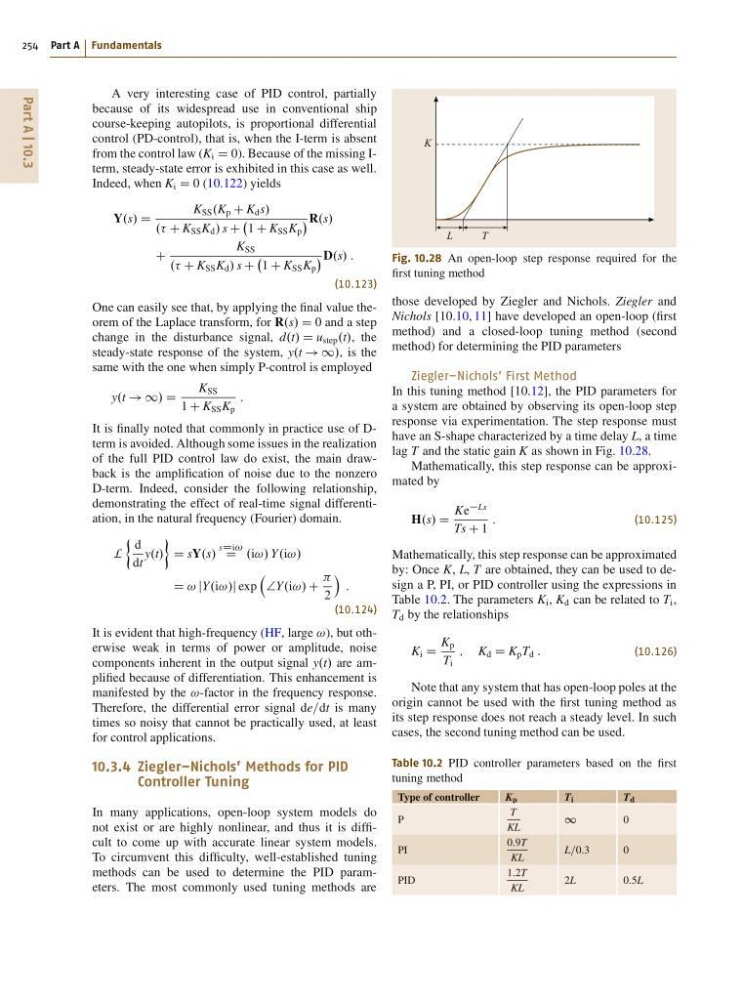
Fig. 10.28 An open-loop step response required for the
first tuning method
those developed by Ziegler and Nichols. Ziegler and
Nichols [10.10, 11] have developed an open-loop (first
method) and a closed-loop tuning method (second
method) for determining the PID parameters
Ziegler–Nichols’ First Method
In this tuning method [10.12], the PID parameters for
a system are obtained by observing its open-loop step
response via experimentation. The step response must
have an S-shape characterized by a time delay L, a time
lag T and the static gain K as shown in Fig. 10.28.
Mathematically, this step response can be approximated by
H.s/ D
Ke
Ls
Ts C 1
:
(10.125)
Mathematically, this step response can be approximated
by: Once K, L, T are obtained, they can be used to design a P, PI, or PID controller using the expressions in
Table 10.2. The parameters K i , K d can be related to T i ,
T d by the relationships
K i D
K p
T i
; K d D K p T d :
(10.126)
Note that any system that has open-loop poles at the
origin cannot be used with the first tuning method as
its step response does not reach a steady level. In such
cases, the second tuning method can be used.
Table 10.2 PID controller parameters based on the first
tuning method
Type of controller
K p
T i
T d
P
T
KL
1
0
PI
0:9T
KL
L=0:3
0
PID
1:2T
KL
2L
0:5L
254 Part A Fundamentals
A very interesting case of PID control, partially
because of its widespread use in conventional ship
course-keeping autopilots, is proportional differential
control (PD-control), that is, when the I-term is absent
from the control law (K i D 0). Because of the missing Iterm, steady-state error is exhibited in this case as well.
Indeed, when K i D 0 (10.122) yields
Y.s/ D
K SS .K p C K d s/
.. C K SS K d / s C
1 C K SS K p
R.s/
C
K SS
.. C K SS K d / s C
1 C K SS K p
D.s/ :
(10.123)
One can easily see that, by applying the final value theorem of the Laplace transform, for R.s/ D 0 and a step
change in the disturbance signal, d.t/ D u step .t/, the
steady-state response of the system, y.t ! 1/, is the
same with the one when simply P-control is employed
y.t ! 1/ D
K SS
1 C K SS K p
:
It is finally noted that commonly in practice use of Dterm is avoided. Although some issues in the realization
of the full PID control law do exist, the main drawback is the amplification of noise due to the nonzero
D-term. Indeed, consider the following relationship,
demonstrating the effect of real-time signal differentiation, in the natural frequency (Fourier) domain.
L
d
dt
y.t/
D sY.s/
sDi!
D .i!/ Y.i!/
D ! jY.i!/j exp
†Y.i!/ C
2
Á
:
(10.124)
It is evident that high-frequency (HF, large !), but otherwise weak in terms of power or amplitude, noise
components inherent in the output signal y.t/ are amplified because of differentiation. This enhancement is
manifested by the !-factor in the frequency response.
Therefore, the differential error signal de=dt is many
times so noisy that cannot be practically used, at least
for control applications.
10.3.4 Ziegler–Nichols’ Methods for PID
Controller Tuning
In many applications, open-loop system models do
not exist or are highly nonlinear, and thus it is difficult to come up with accurate linear system models.
To circumvent this difficulty, well-established tuning
methods can be used to determine the PID parameters. The most commonly used tuning methods are
T
L
K
Fig. 10.28 An open-loop step response required for the
first tuning method
those developed by Ziegler and Nichols. Ziegler and
Nichols [10.10, 11] have developed an open-loop (first
method) and a closed-loop tuning method (second
method) for determining the PID parameters
Ziegler–Nichols’ First Method
In this tuning method [10.12], the PID parameters for
a system are obtained by observing its open-loop step
response via experimentation. The step response must
have an S-shape characterized by a time delay L, a time
lag T and the static gain K as shown in Fig. 10.28.
Mathematically, this step response can be approximated by
H.s/ D
Ke
Ls
Ts C 1
:
(10.125)
Mathematically, this step response can be approximated
by: Once K, L, T are obtained, they can be used to design a P, PI, or PID controller using the expressions in
Table 10.2. The parameters K i , K d can be related to T i ,
T d by the relationships
K i D
K p
T i
; K d D K p T d :
(10.126)
Note that any system that has open-loop poles at the
origin cannot be used with the first tuning method as
its step response does not reach a steady level. In such
cases, the second tuning method can be used.
Table 10.2 PID controller parameters based on the first
tuning method
Type of controller
K p
T i
T d
P
T
KL
1
0
PI
0:9T
KL
L=0:3
0
PID
1:2T
KL
2L
0:5L