

Control Theory and Applications 10.3 SISO System Controls 253
Part A | 10.3
the cases when P and PI-control is employed are as follows
P-control: p c1 .s/ D s C K SS K p C 1 ;
(10.118)
PI-control: p c2 .s/ D s
2
C
K SS K p C 1
s C K SS K i :
(10.119)
In the case that K i D 0 the polynomial in (10.119)
in conjunction with the zero-pole cancellation taking
place in (10.115) for s D 0, (10.119) coincides with the
one in (10.118), that is, the one valid for P-control.
Another interesting case is when
K SS K p C 1
D 0 ,
K p D D1=K SS , when polynomial p c2 .s/ has zero firstorder term. In this case, the closed-loop system poles
are as follows
p 1;2 D ˙
r
K SS K i
:
(10.120)
In conclusion, if K i > 0 (and K SS > 0) the closed-loop
system becomes unstable with one pole in the righthand complex plane, while if K i Ä 0 the closed-loop
system is critically stable with two purely imaginary,
conjugate poles. The analysis above demonstrates the
importance of the proportional term in PI-control for
guaranteeing closed-loop system stability.
The reason for which the PI-control law eliminates
steady-state error is because the transient effect is not
terminated before the output signal coincides with the
setpoint. This is achieved due to the accumulation of
error in the integrator, which, therefore, acts as a memory element in the closed-loop system. In effect, as long
as the error integral is nonzero a persisting control action remains. The tradeoff for this advantage is that
the output may be driven to damped on even sustained
oscillations.
Proportional-Integral-Differential Control
This is the full form of the P-I-D control law. A differential term (D-term) is employed in order to allow us to
deal with some of the problems attributed to the use of
the I-term. One of the most important is the prohibitive
overshoot observed in the closed-loop system response
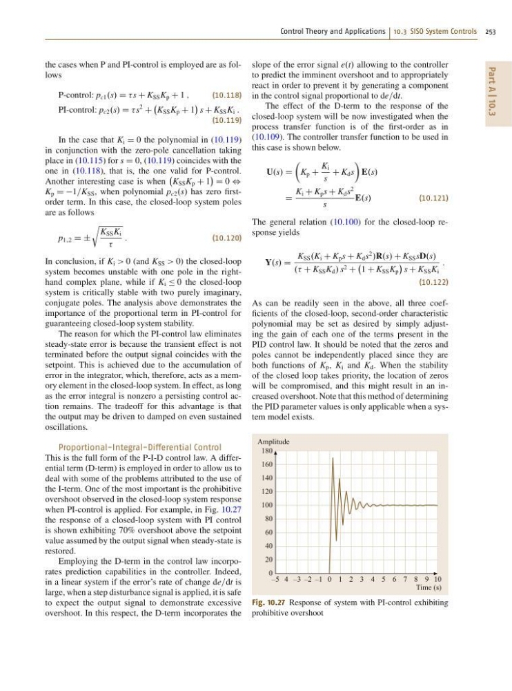
when PI-control is applied. For example, in Fig. 10.27
the response of a closed-loop system with PI control
is shown exhibiting 70% overshoot above the setpoint
value assumed by the output signal when steady-state is
restored.
Employing the D-term in the control law incorporates prediction capabilities in the controller. Indeed,
in a linear system if the error’s rate of change de=dt is
large, when a step disturbance signal is applied, it is safe
to expect the output signal to demonstrate excessive
overshoot. In this respect, the D-term incorporates the
slope of the error signal e.t/ allowing to the controller
to predict the imminent overshoot and to appropriately
react in order to prevent it by generating a component
in the control signal proportional to de=dt.
The effect of the D-term to the response of the
closed-loop system will be now investigated when the
process transfer function is of the first-order as in
(10.109). The controller transfer function to be used in
this case is shown below.
U.s/ D
Â
K p C
K i
s
C K d s
Ã
E.s/
D
K i C K p s C K d s
2
s
E.s/
(10.121)
The general relation (10.100) for the closed-loop response yields
Y.s/ D
K SS .K i C K p s C K d s
2
/R.s/ C K SS sD.s/
.. C K SS K d / s 2 C
1 C K SS K p
s C K SS K i
:
(10.122)
As can be readily seen in the above, all three coefficients of the closed-loop, second-order characteristic
polynomial may be set as desired by simply adjusting the gain of each one of the terms present in the
PID control law. It should be noted that the zeros and
poles cannot be independently placed since they are
both functions of K p , K i and K d . When the stability
of the closed loop takes priority, the location of zeros
will be compromised, and this might result in an increased overshoot. Note that this method of determining
the PID parameter values is only applicable when a system model exists.
–5
Amplitude
1
0
–1
–2
–3
4
2 3 4 5 6 7 8 9 10
Time (s)
180
160
140
120
100
80
60
40
20
0
Fig. 10.27 Response of system with PI-control exhibiting
prohibitive overshoot
Part A | 10.3
the cases when P and PI-control is employed are as follows
P-control: p c1 .s/ D s C K SS K p C 1 ;
(10.118)
PI-control: p c2 .s/ D s
2
C
K SS K p C 1
s C K SS K i :
(10.119)
In the case that K i D 0 the polynomial in (10.119)
in conjunction with the zero-pole cancellation taking
place in (10.115) for s D 0, (10.119) coincides with the
one in (10.118), that is, the one valid for P-control.
Another interesting case is when
K SS K p C 1
D 0 ,
K p D D1=K SS , when polynomial p c2 .s/ has zero firstorder term. In this case, the closed-loop system poles
are as follows
p 1;2 D ˙
r
K SS K i
:
(10.120)
In conclusion, if K i > 0 (and K SS > 0) the closed-loop
system becomes unstable with one pole in the righthand complex plane, while if K i Ä 0 the closed-loop
system is critically stable with two purely imaginary,
conjugate poles. The analysis above demonstrates the
importance of the proportional term in PI-control for
guaranteeing closed-loop system stability.
The reason for which the PI-control law eliminates
steady-state error is because the transient effect is not
terminated before the output signal coincides with the
setpoint. This is achieved due to the accumulation of
error in the integrator, which, therefore, acts as a memory element in the closed-loop system. In effect, as long
as the error integral is nonzero a persisting control action remains. The tradeoff for this advantage is that
the output may be driven to damped on even sustained
oscillations.
Proportional-Integral-Differential Control
This is the full form of the P-I-D control law. A differential term (D-term) is employed in order to allow us to
deal with some of the problems attributed to the use of
the I-term. One of the most important is the prohibitive
overshoot observed in the closed-loop system response
when PI-control is applied. For example, in Fig. 10.27
the response of a closed-loop system with PI control
is shown exhibiting 70% overshoot above the setpoint
value assumed by the output signal when steady-state is
restored.
Employing the D-term in the control law incorporates prediction capabilities in the controller. Indeed,
in a linear system if the error’s rate of change de=dt is
large, when a step disturbance signal is applied, it is safe
to expect the output signal to demonstrate excessive
overshoot. In this respect, the D-term incorporates the
slope of the error signal e.t/ allowing to the controller
to predict the imminent overshoot and to appropriately
react in order to prevent it by generating a component
in the control signal proportional to de=dt.
The effect of the D-term to the response of the
closed-loop system will be now investigated when the
process transfer function is of the first-order as in
(10.109). The controller transfer function to be used in
this case is shown below.
U.s/ D
Â
K p C
K i
s
C K d s
Ã
E.s/
D
K i C K p s C K d s
2
s
E.s/
(10.121)
The general relation (10.100) for the closed-loop response yields
Y.s/ D
K SS .K i C K p s C K d s
2
/R.s/ C K SS sD.s/
.. C K SS K d / s 2 C
1 C K SS K p
s C K SS K i
:
(10.122)
As can be readily seen in the above, all three coefficients of the closed-loop, second-order characteristic
polynomial may be set as desired by simply adjusting the gain of each one of the terms present in the
PID control law. It should be noted that the zeros and
poles cannot be independently placed since they are
both functions of K p , K i and K d . When the stability
of the closed loop takes priority, the location of zeros
will be compromised, and this might result in an increased overshoot. Note that this method of determining
the PID parameter values is only applicable when a system model exists.
–5
Amplitude
1
0
–1
–2
–3
4
2 3 4 5 6 7 8 9 10
Time (s)
180
160
140
120
100
80
60
40
20
0
Fig. 10.27 Response of system with PI-control exhibiting
prohibitive overshoot