

Part A | 10.3
248 Part A Fundamentals
Controller
Process
(or plant)
Process
input
Error
e
Disturbance
d
u
Control
signal
Reference
signal
(setpoint)
r
Response
(or output)
y
Feedback path (or branch)
K (s)
G (s)
Fig. 10.19 Typical block diagram of
a closed-loop system
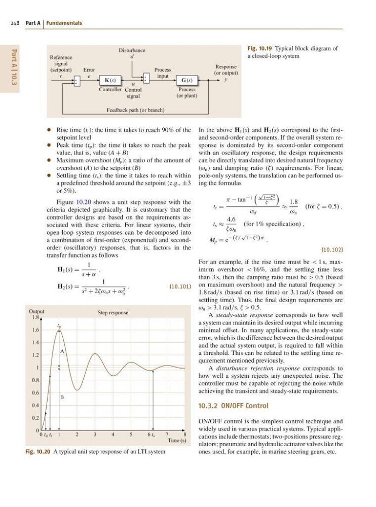
Rise time (t r ): the time it takes to reach 90% of the
setpoint level
Peak time (t p ): the time it takes to reach the peak
value, that is, value (A C B)
Maximum overshoot (M p ): a ratio of the amount of
overshoot (A) to the setpoint (B)
Settling time (t s ): the time it takes to reach within
a predefined threshold around the setpoint (e.g., ˙3
or 5%).
Figure 10.20 shows a unit step response with the
criteria depicted graphically. It is customary that the
controller designs are based on the requirements associated with these criteria. For linear systems, their
open-loop system responses can be decomposed into
a combination of first-order (exponential) and secondorder (oscillatory) responses, that is, factors in the
transfer function as follows
H 1 .s/ D
1
s C ˛
;
H 2 .s/ D
1
s 2 C 2! n s C ! 2
n
:
(10.101)
0
1
B
A
t d
t p
t r
t s
2
3
4
Step response
5
6
7
8
Output
Time (s)
1.8
1.6
1.4
1.2
1
0.8
0.6
0.4
0.2
0
Fig. 10.20 A typical unit step response of an LTI system
In the above H 1 .s/ and H 2 .s/ correspond to the firstand second-order components. If the overall system response is dominated by its second-order component
with an oscillatory response, the design requirements
can be directly translated into desired natural frequency
(! n ) and damping ratio () requirements. For linear,
pole-only systems, the translation can be performed using the formulas
t r D
tan
1
p
1 2
Á
w d
1:8
! n
.for D 0:5/ ;
t s
4:6
! n
.for 1% specification/ ;
M p D e
.=
p
1 2 / :
(10.102)
For an example, if the rise time must be < 1 s, maximum overshoot < 16%, and the settling time less
than 3 s, then the damping ratio must be > 0:5 (based
on maximum overshoot) and the natural frequency >
1:8 rad=s (based on rise time) or 3:1 rad=s (based on
settling time). Thus, the final design requirements are
! n > 3:1 rad=s, > 0:5.
A steady-state response corresponds to how well
a system can maintain its desired output while incurring
minimal offset. In many applications, the steady-state
error, which is the difference between the desired output
and the actual system output, is required to fall within
a threshold. This can be related to the settling time requirement mentioned previously.
A disturbance rejection response corresponds to
how well a system rejects any unexpected noise. The
controller must be capable of rejecting the noise while
achieving the transient and steady-state requirements.
10.3.2 ON/OFF Control
ON/OFF control is the simplest control technique and
widely used in various practical systems. Typical applications include thermostats; two-positions pressure regulators; pneumatic and hydraulic actuator valves like the
ones used, for example, in marine steering gears, etc.
248 Part A Fundamentals
Controller
Process
(or plant)
Process
input
Error
e
Disturbance
d
u
Control
signal
Reference
signal
(setpoint)
r
Response
(or output)
y
Feedback path (or branch)
K (s)
G (s)
Fig. 10.19 Typical block diagram of
a closed-loop system
Rise time (t r ): the time it takes to reach 90% of the
setpoint level
Peak time (t p ): the time it takes to reach the peak
value, that is, value (A C B)
Maximum overshoot (M p ): a ratio of the amount of
overshoot (A) to the setpoint (B)
Settling time (t s ): the time it takes to reach within
a predefined threshold around the setpoint (e.g., ˙3
or 5%).
Figure 10.20 shows a unit step response with the
criteria depicted graphically. It is customary that the
controller designs are based on the requirements associated with these criteria. For linear systems, their
open-loop system responses can be decomposed into
a combination of first-order (exponential) and secondorder (oscillatory) responses, that is, factors in the
transfer function as follows
H 1 .s/ D
1
s C ˛
;
H 2 .s/ D
1
s 2 C 2! n s C ! 2
n
:
(10.101)
0
1
B
A
t d
t p
t r
t s
2
3
4
Step response
5
6
7
8
Output
Time (s)
1.8
1.6
1.4
1.2
1
0.8
0.6
0.4
0.2
0
Fig. 10.20 A typical unit step response of an LTI system
In the above H 1 .s/ and H 2 .s/ correspond to the firstand second-order components. If the overall system response is dominated by its second-order component
with an oscillatory response, the design requirements
can be directly translated into desired natural frequency
(! n ) and damping ratio () requirements. For linear,
pole-only systems, the translation can be performed using the formulas
t r D
tan
1
p
1 2
Á
w d
1:8
! n
.for D 0:5/ ;
t s
4:6
! n
.for 1% specification/ ;
M p D e
.=
p
1 2 / :
(10.102)
For an example, if the rise time must be < 1 s, maximum overshoot < 16%, and the settling time less
than 3 s, then the damping ratio must be > 0:5 (based
on maximum overshoot) and the natural frequency >
1:8 rad=s (based on rise time) or 3:1 rad=s (based on
settling time). Thus, the final design requirements are
! n > 3:1 rad=s, > 0:5.
A steady-state response corresponds to how well
a system can maintain its desired output while incurring
minimal offset. In many applications, the steady-state
error, which is the difference between the desired output
and the actual system output, is required to fall within
a threshold. This can be related to the settling time requirement mentioned previously.
A disturbance rejection response corresponds to
how well a system rejects any unexpected noise. The
controller must be capable of rejecting the noise while
achieving the transient and steady-state requirements.
10.3.2 ON/OFF Control
ON/OFF control is the simplest control technique and
widely used in various practical systems. Typical applications include thermostats; two-positions pressure regulators; pneumatic and hydraulic actuator valves like the
ones used, for example, in marine steering gears, etc.