

Part A | 10.1
236 Part A Fundamentals
The first step toward the linearization of a nonlinear system is to determine the equilibrium points. These
points are defined by the following vector equation
P
x D 0 , f .x 0 ; u 0 / D 0 :
(10.49)
Linearization is then applied around some equilibrium
point .x 0 ; u 0 / by using the Taylor expansions for functions f and g
f .x; u/ f .x 0 ; u 0 / C f
0
x .x 0 ; u 0 / .x x 0 /
C f
0
u .x 0 ; u 0 / .u u 0 /
g .x; u/ g .x 0 ; u 0 / C g
0
x .x 0 ; u 0 / .x x 0 /
C g
0
u .x 0 ; u 0 / .u u 0 / :
(10.50)
In the above, matrices f
0
x .x 0 ; u 0 /, f
0
u .x 0 ; u 0 /, g
0
x .x 0 ; u 0 /,
g
0
u .x 0 ; u 0 / with dimensions n n, n m, p n and p m,
respectively, are defined as follows
f
0
x .x 0 ; u 0 / D
2
6
6
4
@
@x j
f i .x; u/
ˇ
ˇ
ˇ
ˇ
ˇ
ˇ
ˇ
ˇ
x D x 0
u D u 0
; i; j D 1; : : : ; n
3
7
7
5 ;
f
0
u .x 0 ; u 0 / D
2
6
6
4
@
@u j
f i .x; u/
ˇ
ˇ
ˇ
ˇ
ˇ
ˇ
ˇ
ˇ
x D x 0
u D u 0
;
i D 1; : : : ; n
j D 1; : : : ; m
3
7
7
5 ;
(10.51)
g
0
x .x 0 ; u 0 / D
2
6
6
4
@
@x j
g i .x; u/
ˇ
ˇ
ˇ
ˇ
ˇ
ˇ
ˇ
ˇ
x D x 0
u D u 0
;
i D 1; : : : ; p
j D 1; : : : ; n
3
7
7
5 ;
g
0
u .x 0 ; u 0 / D
2
6
6
4
@
@u j
g i .x; u/
ˇ
ˇ
ˇ
ˇ
ˇ
ˇ
ˇ
ˇ
x D x 0
u D u 0
;
i D 1; : : : ; p
j D 1; : : : ; m
3
7
7
5 :
(10.52)
The following change of variables is then adopted
ıx D x x 0 ; ıu D u u 0 ;
ıy D y y 0 D y g .x 0 ; u 0 / :
(10.53)
In effect, the following linearized equations are deduced
for the nonlinear system (10.48) which is valid exclusively in the vicinity of the equilibrium point .x 0 ; u 0 /
ıP x D f
0
x .x 0 ; u 0 / ıx C f
0
u .x 0 ; u 0 / ıu ;
ıy D g
0
x .x 0 ; u 0 / ıx C g
0
u .x 0 ; u 0 / ıu :
(10.54)
Despite its virtues, the technique of linearization has
also a major drawback. This drawback originates from
the fact that the elements of matrices (10.51) and
(10.52) depend on the equilibrium point in the vicinity of which they are calculated. Therefore, a family of
f (x)
x
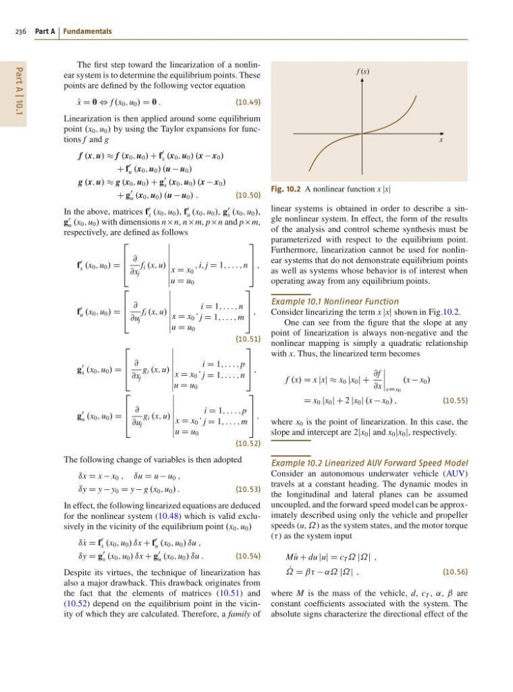
Fig. 10.2 A nonlinear function x jxj
linear systems is obtained in order to describe a single nonlinear system. In effect, the form of the results
of the analysis and control scheme synthesis must be
parameterized with respect to the equilibrium point.
Furthermore, linearization cannot be used for nonlinear systems that do not demonstrate equilibrium points
as well as systems whose behavior is of interest when
operating away from any equilibrium points.
Example 10.1 Nonlinear Function
Consider linearizing the term x jxj shown in Fig.10.2.
One can see from the figure that the slope at any
point of linearization is always non-negative and the
nonlinear mapping is simply a quadratic relationship
with x. Thus, the linearized term becomes
f .x/ D x jxj x 0 jx 0 j C
@f
@x
ˇ
ˇ
ˇ
ˇ
xDx0
.x x 0 /
D x 0 jx 0 j C 2 jx 0 j .x x 0 / ;
(10.55)
where x 0 is the point of linearization. In this case, the
slope and intercept are 2jx 0 j and x 0 jx 0 j, respectively.
Example 10.2 Linearized AUV Forward Speed Model
Consider an autonomous underwater vehicle (AUV)
travels at a constant heading. The dynamic modes in
the longitudinal and lateral planes can be assumed
uncoupled, and the forward speed model can be approximately described using only the vehicle and propeller
speeds (u, ˝) as the system states, and the motor torque
() as the system input
M P
u C du juj D c T ˝ j˝j ;
P
˝ D ˇˇ ˛˝ j˝j ;
(10.56)
where M is the mass of the vehicle, d, c T , ˛, ˇ are
constant coefficients associated with the system. The
absolute signs characterize the directional effect of the
236 Part A Fundamentals
The first step toward the linearization of a nonlinear system is to determine the equilibrium points. These
points are defined by the following vector equation
P
x D 0 , f .x 0 ; u 0 / D 0 :
(10.49)
Linearization is then applied around some equilibrium
point .x 0 ; u 0 / by using the Taylor expansions for functions f and g
f .x; u/ f .x 0 ; u 0 / C f
0
x .x 0 ; u 0 / .x x 0 /
C f
0
u .x 0 ; u 0 / .u u 0 /
g .x; u/ g .x 0 ; u 0 / C g
0
x .x 0 ; u 0 / .x x 0 /
C g
0
u .x 0 ; u 0 / .u u 0 / :
(10.50)
In the above, matrices f
0
x .x 0 ; u 0 /, f
0
u .x 0 ; u 0 /, g
0
x .x 0 ; u 0 /,
g
0
u .x 0 ; u 0 / with dimensions n n, n m, p n and p m,
respectively, are defined as follows
f
0
x .x 0 ; u 0 / D
2
6
6
4
@
@x j
f i .x; u/
ˇ
ˇ
ˇ
ˇ
ˇ
ˇ
ˇ
ˇ
x D x 0
u D u 0
; i; j D 1; : : : ; n
3
7
7
5 ;
f
0
u .x 0 ; u 0 / D
2
6
6
4
@
@u j
f i .x; u/
ˇ
ˇ
ˇ
ˇ
ˇ
ˇ
ˇ
ˇ
x D x 0
u D u 0
;
i D 1; : : : ; n
j D 1; : : : ; m
3
7
7
5 ;
(10.51)
g
0
x .x 0 ; u 0 / D
2
6
6
4
@
@x j
g i .x; u/
ˇ
ˇ
ˇ
ˇ
ˇ
ˇ
ˇ
ˇ
x D x 0
u D u 0
;
i D 1; : : : ; p
j D 1; : : : ; n
3
7
7
5 ;
g
0
u .x 0 ; u 0 / D
2
6
6
4
@
@u j
g i .x; u/
ˇ
ˇ
ˇ
ˇ
ˇ
ˇ
ˇ
ˇ
x D x 0
u D u 0
;
i D 1; : : : ; p
j D 1; : : : ; m
3
7
7
5 :
(10.52)
The following change of variables is then adopted
ıx D x x 0 ; ıu D u u 0 ;
ıy D y y 0 D y g .x 0 ; u 0 / :
(10.53)
In effect, the following linearized equations are deduced
for the nonlinear system (10.48) which is valid exclusively in the vicinity of the equilibrium point .x 0 ; u 0 /
ıP x D f
0
x .x 0 ; u 0 / ıx C f
0
u .x 0 ; u 0 / ıu ;
ıy D g
0
x .x 0 ; u 0 / ıx C g
0
u .x 0 ; u 0 / ıu :
(10.54)
Despite its virtues, the technique of linearization has
also a major drawback. This drawback originates from
the fact that the elements of matrices (10.51) and
(10.52) depend on the equilibrium point in the vicinity of which they are calculated. Therefore, a family of
f (x)
x
Fig. 10.2 A nonlinear function x jxj
linear systems is obtained in order to describe a single nonlinear system. In effect, the form of the results
of the analysis and control scheme synthesis must be
parameterized with respect to the equilibrium point.
Furthermore, linearization cannot be used for nonlinear systems that do not demonstrate equilibrium points
as well as systems whose behavior is of interest when
operating away from any equilibrium points.
Example 10.1 Nonlinear Function
Consider linearizing the term x jxj shown in Fig.10.2.
One can see from the figure that the slope at any
point of linearization is always non-negative and the
nonlinear mapping is simply a quadratic relationship
with x. Thus, the linearized term becomes
f .x/ D x jxj x 0 jx 0 j C
@f
@x
ˇ
ˇ
ˇ
ˇ
xDx0
.x x 0 /
D x 0 jx 0 j C 2 jx 0 j .x x 0 / ;
(10.55)
where x 0 is the point of linearization. In this case, the
slope and intercept are 2jx 0 j and x 0 jx 0 j, respectively.
Example 10.2 Linearized AUV Forward Speed Model
Consider an autonomous underwater vehicle (AUV)
travels at a constant heading. The dynamic modes in
the longitudinal and lateral planes can be assumed
uncoupled, and the forward speed model can be approximately described using only the vehicle and propeller
speeds (u, ˝) as the system states, and the motor torque
() as the system input
M P
u C du juj D c T ˝ j˝j ;
P
˝ D ˇˇ ˛˝ j˝j ;
(10.56)
where M is the mass of the vehicle, d, c T , ˛, ˇ are
constant coefficients associated with the system. The
absolute signs characterize the directional effect of the