

Control Theory and Applications 10.1 System Theory 231
Part A | 10.1
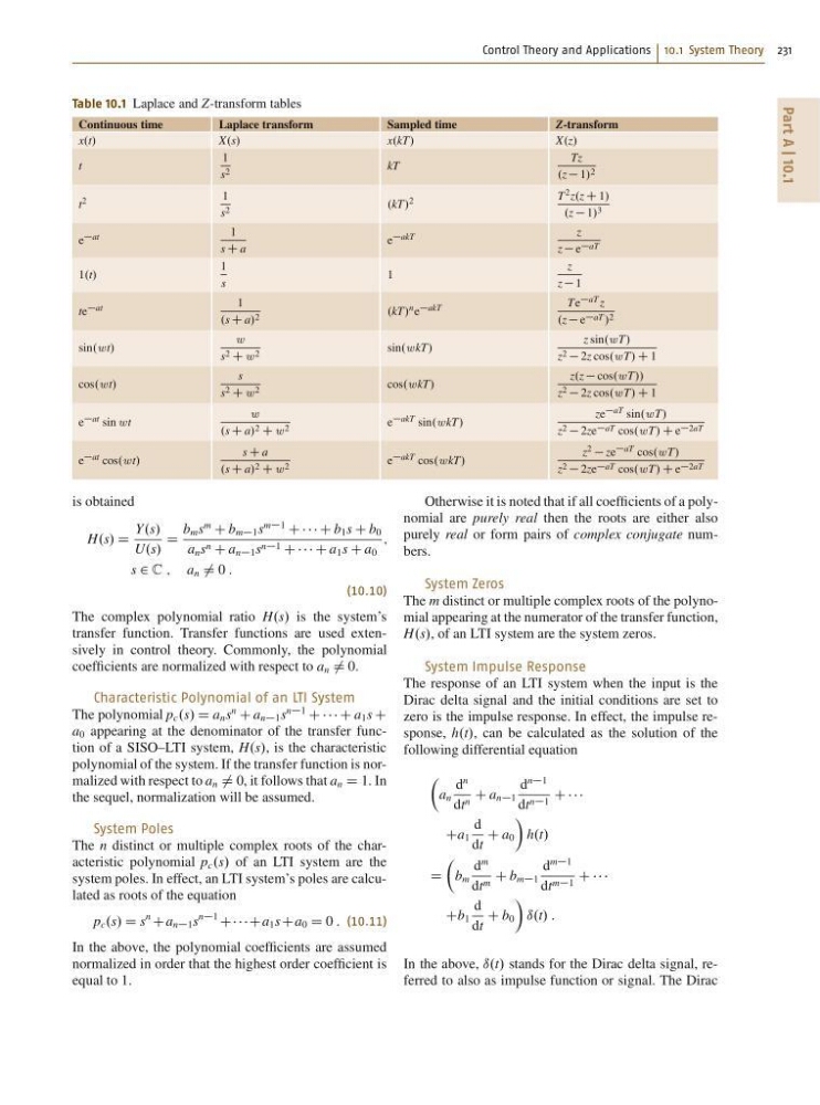
Table 10.1 Laplace and Z-transform tables
Continuous time
Laplace transform
Sampled time
Z-transform
x.t/
X.s/
x.kT/
X.z/
t
1
s 2
kT
Tz
.z 1/ 2
t 2
1
s 2
.kT/ 2
T
2 z.z C 1/
.z 1/ 3
e at
1
s C a
e akT
z
z e aT
1.t/
1
s
1
z
z 1
te at
1
.s C a/ 2
.kT/ n e akT
Te aT z
.z e aT / 2
sin.w t/
w
s 2 C w 2
sin.w kT/
z sin.w T/
z 2 2z cos.w T/ C 1
cos.w t/
s
s 2 C w 2
cos.w kT/
z.z cos.w T//
z 2 2z cos.w T/ C 1
e at sin w t
w
.s C a/ 2 C w 2
e akT sin.w kT/
ze aT sin.w T/
z 2 2ze aT cos.w T/ C e 2aT
e at cos.w t/
s C a
.s C a/ 2 C w 2
e akT cos.w kT/
z 2 ze aT cos.w T/
z 2 2ze aT cos.w T/ C e 2aT
is obtained
H.s/ D
Y.s/
U.s/
D
b m s
m
C b m1 s
m1
C C C C C b 1 s C b 0
a n s n C a n1 s n1 C C C C C a 1 s C a 0
;
s 2 C ; a n ¤ 0 :
(10.10)
The complex polynomial ratio H.s/ is the system’s
transfer function. Transfer functions are used extensively in control theory. Commonly, the polynomial
coefficients are normalized with respect to a n ¤ 0.
Characteristic Polynomial of an LTI System
The polynomial p c .s/ D a n s
n
C a n1 s
n1
C C C C C a 1 s C
a 0 appearing at the denominator of the transfer function of a SISO–LTI system, H.s/, is the characteristic
polynomial of the system. If the transfer function is normalized with respect to a n ¤ 0, it follows that a n D 1. In
the sequel, normalization will be assumed.
System Poles
The n distinct or multiple complex roots of the characteristic polynomial p c .s/ of an LTI system are the
system poles. In effect, an LTI system’s poles are calculated as roots of the equation
p c .s/ D s
n
Ca n1 s
n1
CC C CCa 1 sCa 0 D 0 : (10.11)
In the above, the polynomial coefficients are assumed
normalized in order that the highest order coefficient is
equal to 1.
Otherwise it is noted that if all coefficients of a polynomial are purely real then the roots are either also
purely real or form pairs of complex conjugate numbers.
System Zeros
The m distinct or multiple complex roots of the polynomial appearing at the numerator of the transfer function,
H.s/, of an LTI system are the system zeros.
System Impulse Response
The response of an LTI system when the input is the
Dirac delta signal and the initial conditions are set to
zero is the impulse response. In effect, the impulse response, h.t/, can be calculated as the solution of the
following differential equation
Â
a n
d
n
dt n C a n1
d
n1
dt n1 C C C C
Ca 1
d
dt
C a 0
Ã
h.t/
D
Â
b m
d
m
dt m C b m1
d
m1
dt m1 C C C C
Cb 1
d
dt
C b 0
Ã
ı.t/ :
In the above, ı.t/ stands for the Dirac delta signal, referred to also as impulse function or signal. The Dirac
Part A | 10.1
Table 10.1 Laplace and Z-transform tables
Continuous time
Laplace transform
Sampled time
Z-transform
x.t/
X.s/
x.kT/
X.z/
t
1
s 2
kT
Tz
.z 1/ 2
t 2
1
s 2
.kT/ 2
T
2 z.z C 1/
.z 1/ 3
e at
1
s C a
e akT
z
z e aT
1.t/
1
s
1
z
z 1
te at
1
.s C a/ 2
.kT/ n e akT
Te aT z
.z e aT / 2
sin.w t/
w
s 2 C w 2
sin.w kT/
z sin.w T/
z 2 2z cos.w T/ C 1
cos.w t/
s
s 2 C w 2
cos.w kT/
z.z cos.w T//
z 2 2z cos.w T/ C 1
e at sin w t
w
.s C a/ 2 C w 2
e akT sin.w kT/
ze aT sin.w T/
z 2 2ze aT cos.w T/ C e 2aT
e at cos.w t/
s C a
.s C a/ 2 C w 2
e akT cos.w kT/
z 2 ze aT cos.w T/
z 2 2ze aT cos.w T/ C e 2aT
is obtained
H.s/ D
Y.s/
U.s/
D
b m s
m
C b m1 s
m1
C C C C C b 1 s C b 0
a n s n C a n1 s n1 C C C C C a 1 s C a 0
;
s 2 C ; a n ¤ 0 :
(10.10)
The complex polynomial ratio H.s/ is the system’s
transfer function. Transfer functions are used extensively in control theory. Commonly, the polynomial
coefficients are normalized with respect to a n ¤ 0.
Characteristic Polynomial of an LTI System
The polynomial p c .s/ D a n s
n
C a n1 s
n1
C C C C C a 1 s C
a 0 appearing at the denominator of the transfer function of a SISO–LTI system, H.s/, is the characteristic
polynomial of the system. If the transfer function is normalized with respect to a n ¤ 0, it follows that a n D 1. In
the sequel, normalization will be assumed.
System Poles
The n distinct or multiple complex roots of the characteristic polynomial p c .s/ of an LTI system are the
system poles. In effect, an LTI system’s poles are calculated as roots of the equation
p c .s/ D s
n
Ca n1 s
n1
CC C CCa 1 sCa 0 D 0 : (10.11)
In the above, the polynomial coefficients are assumed
normalized in order that the highest order coefficient is
equal to 1.
Otherwise it is noted that if all coefficients of a polynomial are purely real then the roots are either also
purely real or form pairs of complex conjugate numbers.
System Zeros
The m distinct or multiple complex roots of the polynomial appearing at the numerator of the transfer function,
H.s/, of an LTI system are the system zeros.
System Impulse Response
The response of an LTI system when the input is the
Dirac delta signal and the initial conditions are set to
zero is the impulse response. In effect, the impulse response, h.t/, can be calculated as the solution of the
following differential equation
Â
a n
d
n
dt n C a n1
d
n1
dt n1 C C C C
Ca 1
d
dt
C a 0
Ã
h.t/
D
Â
b m
d
m
dt m C b m1
d
m1
dt m1 C C C C
Cb 1
d
dt
C b 0
Ã
ı.t/ :
In the above, ı.t/ stands for the Dirac delta signal, referred to also as impulse function or signal. The Dirac