

Control Theory and Applications 10.1 System Theory 229
Part A | 10.1
Before embarking on the methods to develop a control system, a clear understanding of the behavior and
analysis of the response of the plant is needed. This
is commonly achieved by developing a mathematical
model of the system. The type and the complexity
of such a model, though, depend on various salient
features of the plant in hand. One of the most important features is whether the plant is static or dynamic.
A static system is one for which the output signal values
at any given time instant can be determined by employing exclusively the input signal values at the exact same
time instant. In effect, static systems are commonly described by algebraic equations of the following general
form
y D f .u/ :
(10.1)
In the above, u and y are the input and output signals,
respectively, conveniently packed in vectors.
Another class of systems, though, which is usually
the case in feedback control theory and engineering,
are dynamic systems. A dynamic system is described
by a number of dynamic equations, integro-differential
equations including at least time as an independent variable. Specifically, the description of a dynamic system
must encompass all the constraint equations as well as
the full set of initial, or in some cases, final conditions
required for the determination of a special solution of
the integro-differential equations. A deeper insight in
this definition as well as the fundamental description
methods for linear and time-invariant dynamic systems
is presented in the remainder of this chapter.
10.1.2 The Laplace Transform
The Laplace transform is a linear integral transform that
is defined as follows for a signal x.t/
X.s/ D L fx.t/g D
1
Z
0
x.t/e
st dt :
(10.2)
The (one-sided) Laplace transform is used extensively
for analyses of either signals or systems in the complex
frequency domain, s D a C i!. The complex frequency
comes as generalization of the (natural) frequency as
defined especially for periodic signals, sinusoidal signals, or sums of such. This is manifested also by the
fact that the Fourier transformation of any signal can be
derived by substituting s D i! in its Laplace transformation or equivalently setting a D 0. These remarks are
investigated in the following example.
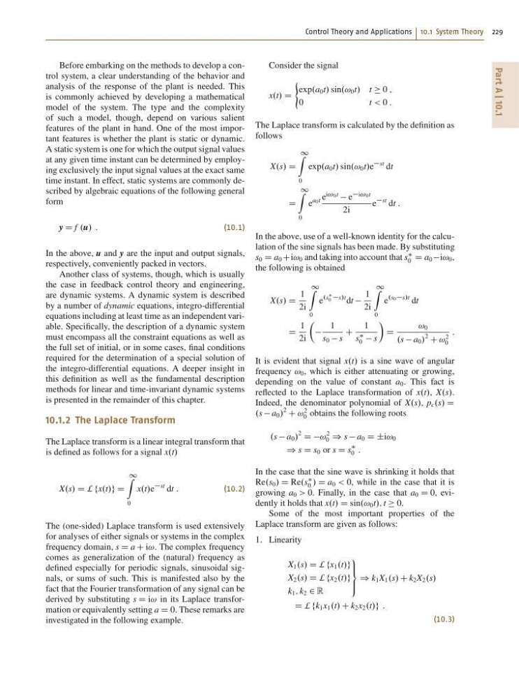
Consider the signal
x.t/ D
(
exp.a 0 t/ sin.! 0 t/ t 0 ;
0
t < 0 :
The Laplace transform is calculated by the definition as
follows
X.s/ D
1
Z
0
exp.a 0 t/ sin.! 0 t/e
st dt
D
1
Z
0
e
a0t e
i!0t
e
i!0t
2i
e
st dt :
In the above, use of a well-known identity for the calculation of the sine signals has been made. By substituting
s 0 D a 0 Ci! 0 and taking into account that s
0 D a 0 i! 0 ,
the following is obtained
X.s/ D
1
2i
1
Z
0
e
.s
0 s/t dt
1
2i
1
Z
0
e
.s0s/t dt
D
1
2i
Â
1
s 0 s
C
1
s
0 s
Ã
D
! 0
.s a 0 /
2 C !
2
0
:
It is evident that signal x.t/ is a sine wave of angular
frequency ! 0 , which is either attenuating or growing,
depending on the value of constant a 0 . This fact is
reflected to the Laplace transformation of x.t/, X.s/.
Indeed, the denominator polynomial of X.s/, p c .s/ D
.s a 0 /
2 C !
2
0 obtains the following roots
.s a 0 /
2 D D!
2
0 ) s a 0 D ˙i! 0
) s D s 0 or s D s
0 :
In the case that the sine wave is shrinking it holds that
Re.s 0 / D Re.s
0 / D a 0 < 0, while in the case that it is
growing a 0 > 0. Finally, in the case that a 0 D 0, evidently it holds that x.t/ D sin.! 0 t/; t 0.
Some of the most important properties of the
Laplace transform are given as follows:
1. Linearity
X 1 .s/ D L fx 1 .t/g
X 2 .s/ D L fx 2 .t/g
k 1 ; k 2 2 R
9
> =
> ;
) k 1 X 1 .s/ C k 2 X 2 .s/
D L fk 1 x 1 .t/ C k 2 x 2 .t/g :
(10.3)
Part A | 10.1
Before embarking on the methods to develop a control system, a clear understanding of the behavior and
analysis of the response of the plant is needed. This
is commonly achieved by developing a mathematical
model of the system. The type and the complexity
of such a model, though, depend on various salient
features of the plant in hand. One of the most important features is whether the plant is static or dynamic.
A static system is one for which the output signal values
at any given time instant can be determined by employing exclusively the input signal values at the exact same
time instant. In effect, static systems are commonly described by algebraic equations of the following general
form
y D f .u/ :
(10.1)
In the above, u and y are the input and output signals,
respectively, conveniently packed in vectors.
Another class of systems, though, which is usually
the case in feedback control theory and engineering,
are dynamic systems. A dynamic system is described
by a number of dynamic equations, integro-differential
equations including at least time as an independent variable. Specifically, the description of a dynamic system
must encompass all the constraint equations as well as
the full set of initial, or in some cases, final conditions
required for the determination of a special solution of
the integro-differential equations. A deeper insight in
this definition as well as the fundamental description
methods for linear and time-invariant dynamic systems
is presented in the remainder of this chapter.
10.1.2 The Laplace Transform
The Laplace transform is a linear integral transform that
is defined as follows for a signal x.t/
X.s/ D L fx.t/g D
1
Z
0
x.t/e
st dt :
(10.2)
The (one-sided) Laplace transform is used extensively
for analyses of either signals or systems in the complex
frequency domain, s D a C i!. The complex frequency
comes as generalization of the (natural) frequency as
defined especially for periodic signals, sinusoidal signals, or sums of such. This is manifested also by the
fact that the Fourier transformation of any signal can be
derived by substituting s D i! in its Laplace transformation or equivalently setting a D 0. These remarks are
investigated in the following example.
Consider the signal
x.t/ D
(
exp.a 0 t/ sin.! 0 t/ t 0 ;
0
t < 0 :
The Laplace transform is calculated by the definition as
follows
X.s/ D
1
Z
0
exp.a 0 t/ sin.! 0 t/e
st dt
D
1
Z
0
e
a0t e
i!0t
e
i!0t
2i
e
st dt :
In the above, use of a well-known identity for the calculation of the sine signals has been made. By substituting
s 0 D a 0 Ci! 0 and taking into account that s
0 D a 0 i! 0 ,
the following is obtained
X.s/ D
1
2i
1
Z
0
e
.s
0 s/t dt
1
2i
1
Z
0
e
.s0s/t dt
D
1
2i
Â
1
s 0 s
C
1
s
0 s
Ã
D
! 0
.s a 0 /
2 C !
2
0
:
It is evident that signal x.t/ is a sine wave of angular
frequency ! 0 , which is either attenuating or growing,
depending on the value of constant a 0 . This fact is
reflected to the Laplace transformation of x.t/, X.s/.
Indeed, the denominator polynomial of X.s/, p c .s/ D
.s a 0 /
2 C !
2
0 obtains the following roots
.s a 0 /
2 D D!
2
0 ) s a 0 D ˙i! 0
) s D s 0 or s D s
0 :
In the case that the sine wave is shrinking it holds that
Re.s 0 / D Re.s
0 / D a 0 < 0, while in the case that it is
growing a 0 > 0. Finally, in the case that a 0 D 0, evidently it holds that x.t/ D sin.! 0 t/; t 0.
Some of the most important properties of the
Laplace transform are given as follows:
1. Linearity
X 1 .s/ D L fx 1 .t/g
X 2 .s/ D L fx 2 .t/g
k 1 ; k 2 2 R
9
> =
> ;
) k 1 X 1 .s/ C k 2 X 2 .s/
D L fk 1 x 1 .t/ C k 2 x 2 .t/g :
(10.3)