

Digital Signal Processing 9.5 Optimal Signal Estimation 223
Part A | 9.5
As can be seen a known, in this case, the LTI-SISO
system is driven by an unknown (to be estimated) x.t/.
or the known LTI system, the transfer function G.s/,
in the complex frequency (Laplace) domain, or G.!/,
in the Fourier (frequency) domain, or equivalently its
impulse response g.t/ in the time domain is assumed
known. Such an LTI system may model a measurement
instrument, or sensor, or transducer, or telecommunications receiver.
Then, a linear filter with transfer function H.s/ is
sought that will receive as input the noisy instrument
response w .t/ and output waveform y.t/, which is expected to be the optimum, in the mean square sense,
estimate of the unknown waveform x.t/.
The objective is to determine transfer function H.s/,
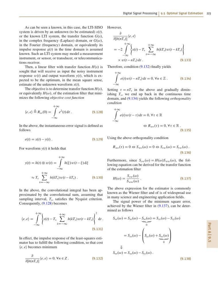
or equivalently H.!/, of the estimation filter that minimizes the following objective cost function
he; ei , R ee .0/ D
C1 Z
1
e
2
.t/ dt :
(9.128)
In the above, the instantaneous error signal is defined as
follows
e.t/ D x.t/ y.t/ :
(9.129)
For waveform y.t/ it holds that
y.t/ D h.t/ ˝ w .t/ D
C1 Z
1
h../w .t / d
T s
C1 X
kDD1
h.kT s /w .t kT s / :
(9.130)
In the above, the convolutional integral has been approximated by the convolutional sum, assuming that
sampling interval, T s , satisfies the Nyquist criterion.
Consequently, (9.128) becomes
he; ei D
C1 Z
1
(
x.t/ T s
C1 X
kDD1
h.kT s /w .t kT s /
)2
dt :
(9.131)
In effect, the impulse response of the least-squares estimator has to fulfill the following condition, so that cost
he; ei becomes minimum
@
@Œh.nT s /
he; ei D 0; 8n 2 Z :
(9.132)
However,
@
@Œh.nT s /
he; ei
D D2
C1 Z
1
(
x.t/ T s
C1 X
kDD1
h.kT s /w .t kT s /
)
w .t nT s / dt :
(9.133)
Therefore, condition (9.132) finally yields
C1 Z
1
e.t/w .t nT s / dt D 0; 8n 2 Z :
(9.134)
Setting D nT s in the above and gradually diminishing T s , we end up back in the continuous time
domain, and (9.134) yields the following orthogonality
condition
C1 Z
1
e.t/w .t / dt D 0; 8 2 R
, R we ../ D 0; 8 2 R :
(9.135)
Using the above orthogonality condition
R we ../ D 0 , S we .!/ D 0 , S xw .!/ D S yw .!/ :
(9.136)
Furthermore, since S yw .!/ D H.!/S ww .!/, the following equation can be derived for the transfer function
of the estimation filter
H.!/ D
S xw .!/
S ww .!/
:
(9.137)
The above expression for the estimator is commonly
known as the Wiener filter and of is of widespread use
in many science and engineering application fields.
The signal power of the minimum square error,
achieved by the Wiener filter in (9.137), can be determined as follows
S ee .!/ D S xe .!/ S ye .!/
„ƒ‚…
0
D S xx .!/ S xy .!/
D S xx .!/
0
B
@Syy.!/ C S ey .!/
„ƒ‚…
0
1
C
A
+
S ee .!/ D S xx .!/ S yy .!/ :
(9.138)
Part A | 9.5
As can be seen a known, in this case, the LTI-SISO
system is driven by an unknown (to be estimated) x.t/.
or the known LTI system, the transfer function G.s/,
in the complex frequency (Laplace) domain, or G.!/,
in the Fourier (frequency) domain, or equivalently its
impulse response g.t/ in the time domain is assumed
known. Such an LTI system may model a measurement
instrument, or sensor, or transducer, or telecommunications receiver.
Then, a linear filter with transfer function H.s/ is
sought that will receive as input the noisy instrument
response w .t/ and output waveform y.t/, which is expected to be the optimum, in the mean square sense,
estimate of the unknown waveform x.t/.
The objective is to determine transfer function H.s/,
or equivalently H.!/, of the estimation filter that minimizes the following objective cost function
he; ei , R ee .0/ D
C1 Z
1
e
2
.t/ dt :
(9.128)
In the above, the instantaneous error signal is defined as
follows
e.t/ D x.t/ y.t/ :
(9.129)
For waveform y.t/ it holds that
y.t/ D h.t/ ˝ w .t/ D
C1 Z
1
h../w .t / d
T s
C1 X
kDD1
h.kT s /w .t kT s / :
(9.130)
In the above, the convolutional integral has been approximated by the convolutional sum, assuming that
sampling interval, T s , satisfies the Nyquist criterion.
Consequently, (9.128) becomes
he; ei D
C1 Z
1
(
x.t/ T s
C1 X
kDD1
h.kT s /w .t kT s /
)2
dt :
(9.131)
In effect, the impulse response of the least-squares estimator has to fulfill the following condition, so that cost
he; ei becomes minimum
@
@Œh.nT s /
he; ei D 0; 8n 2 Z :
(9.132)
However,
@
@Œh.nT s /
he; ei
D D2
C1 Z
1
(
x.t/ T s
C1 X
kDD1
h.kT s /w .t kT s /
)
w .t nT s / dt :
(9.133)
Therefore, condition (9.132) finally yields
C1 Z
1
e.t/w .t nT s / dt D 0; 8n 2 Z :
(9.134)
Setting D nT s in the above and gradually diminishing T s , we end up back in the continuous time
domain, and (9.134) yields the following orthogonality
condition
C1 Z
1
e.t/w .t / dt D 0; 8 2 R
, R we ../ D 0; 8 2 R :
(9.135)
Using the above orthogonality condition
R we ../ D 0 , S we .!/ D 0 , S xw .!/ D S yw .!/ :
(9.136)
Furthermore, since S yw .!/ D H.!/S ww .!/, the following equation can be derived for the transfer function
of the estimation filter
H.!/ D
S xw .!/
S ww .!/
:
(9.137)
The above expression for the estimator is commonly
known as the Wiener filter and of is of widespread use
in many science and engineering application fields.
The signal power of the minimum square error,
achieved by the Wiener filter in (9.137), can be determined as follows
S ee .!/ D S xe .!/ S ye .!/
„ƒ‚…
0
D S xx .!/ S xy .!/
D S xx .!/
0
B
@Syy.!/ C S ey .!/
„ƒ‚…
0
1
C
A
+
S ee .!/ D S xx .!/ S yy .!/ :
(9.138)