

Digital Signal Processing 9.3 The Fast Fourier Transform (FFT) 213
Part A | 9.3
Table 9.3 8-point DFT (N D 8)
X.k/ D
1
N
N1 X
nD0
x.n/e
i2 nk
N
D
1
N
N1 X
nD0
x.n/W N
nk W N D e
i2
N
X.0/ D x.0/W
0
8 C x.1/W
0
8 C x.2/W
0
8 C x.3/W
0
8 C x.4/W
0
8 C x.5/W
0
8 C x.6/W
0
8 C x.7/W
0
8
X.1/ D x.0/W
0
8 C x.1/W
1
8 C x.2/W
2
8 C x.3/W
3
8 C x.4/W
4
8 C x.5/W
5
8 C x.6/W
6
8 C x.7/W
7
8
X.2/ D x.0/W
0
8 C x.1/W
2
8 C x.2/W
4
8 C x.3/W
6
8 C x.4/W
8
8 C x.5/W
10
8 C x.6/W
12
8 C x.7/W
14
8
X.3/ D x.0/W
0
8 C x.1/W
3
8 C x.2/W
6
8 C x.3/W
9
8 C x.4/W
12
8 C x.5/W
15
8 C x.6/W
18
8 C x.7/W
21
8
X.4/ D x.0/W
0
8 C x.1/W
4
8 C x.2/W
8
8 C x.3/W
12
8 C x.4/W
16
8 C x.5/W
20
8 C x.6/W
24
8 C x.7/W
28
8
X.5/ D x.0/W
0
8 C x.1/W
5
8 C x.2/W
10
8 C x.3/W
15
8 C x.4/W
20
8 C x.5/W
25
8 C x.6/W
30
8 C x.7/W
35
8
X.6/ D x.0/W
0
8 C x.1/W
6
8 C x.2/W
12
8 C x.3/W
18
8 C x.4/W
24
8 C x.5/W
30
8 C x.6/W
36
8 C x.7/W
42
8
X.7/ D x.0/W
0
8 C x.1/W
7
8 C x.2/W
14
8 C x.3/W
21
8 C x.4/W
28
8 C x.5/W
35
8 C x.6/W
42
8 C x.7/W
49
8
N 2 Complex multiplications
1
N
Scaling factor omitted
Table 9.4 8-point DFT. Applying the properties of symmetry and periodicity to W
r
N for N D 8
W
4
8 D W
0C4
8
D DW
0
8 D D1
W
5
8 D W
1C4
8
D DW
1
8
W
6
8 D W
2C4
8
D DW
2
8
N D 8
W
7
8 D W
3C4
8
D DW
3
8
W
8
8 D W
0C8
8
D CW
0
8 D C1
W
9
8 D W
1C8
8
D CW
1
8
W
10
8 D W
2C8
8
D CW
2
8
W
11
8 D W
3C4
8
D CW
3
8
Symmetry: W
rCN=2
N
D DW
r
N , Periodicity: W
rCN
N
D W
r
N
dition, the German mathematician Carl Friedrich Gauss
(1777–1855) had used the method more than a century
earlier.
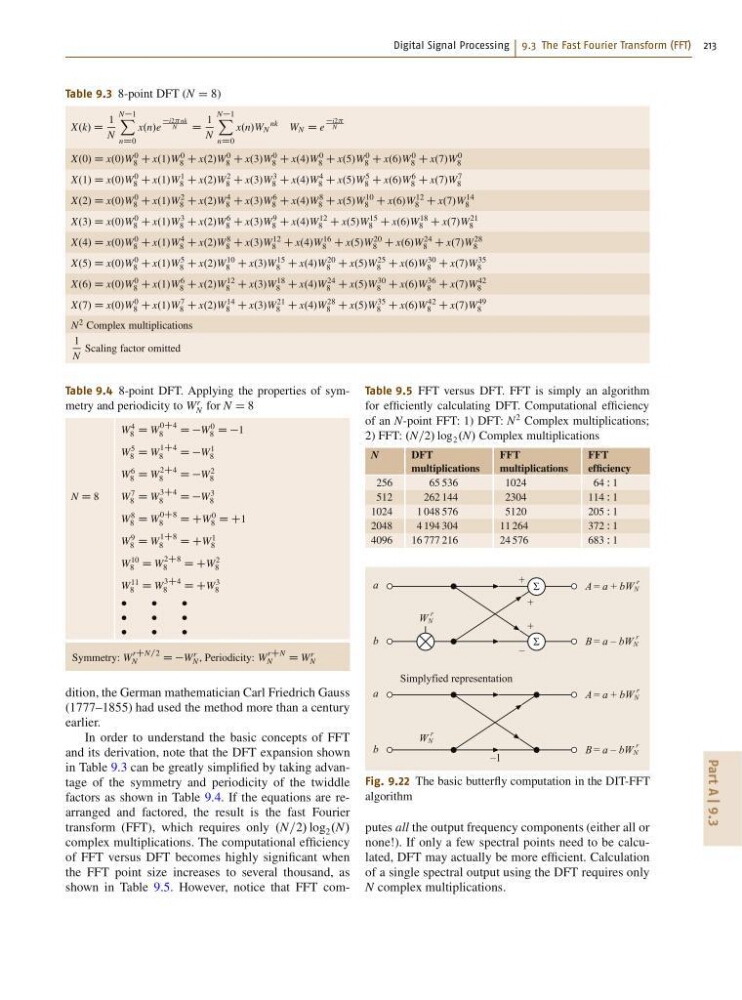
In order to understand the basic concepts of FFT
and its derivation, note that the DFT expansion shown
in Table 9.3 can be greatly simplified by taking advantage of the symmetry and periodicity of the twiddle
factors as shown in Table 9.4. If the equations are rearranged and factored, the result is the fast Fourier
transform (FFT), which requires only .N=2/ log 2 .N/
complex multiplications. The computational efficiency
of FFT versus DFT becomes highly significant when
the FFT point size increases to several thousand, as
shown in Table 9.5. However, notice that FFT comTable 9.5 FFT versus DFT. FFT is simply an algorithm
for efficiently calculating DFT. Computational efficiency
of an N-point FFT: 1) DFT: N
2 Complex multiplications;
2) FFT: .N=2/ log 2 .N/ Complex multiplications
N
DFT
multiplications
FFT
multiplications
FFT
efficiency
256
65 536
1024
64 W 1
512
262 144
2304
114 W 1
1024
1 048 576
5120
205 W 1
2048
4 194 304
11 264
372 W 1
4096
16 777 216
24 576
683 W 1
a
A = a + bW N
r
+
+
+
Σ
b
B = a – bW N
r
–
–1
Σ
W N
r
a
Simplyfied representation
A = a + bW N
r
b
B = a – bW N
r
W N
r
Fig. 9.22 The basic butterfly computation in the DIT-FFT
algorithm
putes all the output frequency components (either all or
none!). If only a few spectral points need to be calculated, DFT may actually be more efficient. Calculation
of a single spectral output using the DFT requires only
N complex multiplications.
Part A | 9.3
Table 9.3 8-point DFT (N D 8)
X.k/ D
1
N
N1 X
nD0
x.n/e
i2 nk
N
D
1
N
N1 X
nD0
x.n/W N
nk W N D e
i2
N
X.0/ D x.0/W
0
8 C x.1/W
0
8 C x.2/W
0
8 C x.3/W
0
8 C x.4/W
0
8 C x.5/W
0
8 C x.6/W
0
8 C x.7/W
0
8
X.1/ D x.0/W
0
8 C x.1/W
1
8 C x.2/W
2
8 C x.3/W
3
8 C x.4/W
4
8 C x.5/W
5
8 C x.6/W
6
8 C x.7/W
7
8
X.2/ D x.0/W
0
8 C x.1/W
2
8 C x.2/W
4
8 C x.3/W
6
8 C x.4/W
8
8 C x.5/W
10
8 C x.6/W
12
8 C x.7/W
14
8
X.3/ D x.0/W
0
8 C x.1/W
3
8 C x.2/W
6
8 C x.3/W
9
8 C x.4/W
12
8 C x.5/W
15
8 C x.6/W
18
8 C x.7/W
21
8
X.4/ D x.0/W
0
8 C x.1/W
4
8 C x.2/W
8
8 C x.3/W
12
8 C x.4/W
16
8 C x.5/W
20
8 C x.6/W
24
8 C x.7/W
28
8
X.5/ D x.0/W
0
8 C x.1/W
5
8 C x.2/W
10
8 C x.3/W
15
8 C x.4/W
20
8 C x.5/W
25
8 C x.6/W
30
8 C x.7/W
35
8
X.6/ D x.0/W
0
8 C x.1/W
6
8 C x.2/W
12
8 C x.3/W
18
8 C x.4/W
24
8 C x.5/W
30
8 C x.6/W
36
8 C x.7/W
42
8
X.7/ D x.0/W
0
8 C x.1/W
7
8 C x.2/W
14
8 C x.3/W
21
8 C x.4/W
28
8 C x.5/W
35
8 C x.6/W
42
8 C x.7/W
49
8
N 2 Complex multiplications
1
N
Scaling factor omitted
Table 9.4 8-point DFT. Applying the properties of symmetry and periodicity to W
r
N for N D 8
W
4
8 D W
0C4
8
D DW
0
8 D D1
W
5
8 D W
1C4
8
D DW
1
8
W
6
8 D W
2C4
8
D DW
2
8
N D 8
W
7
8 D W
3C4
8
D DW
3
8
W
8
8 D W
0C8
8
D CW
0
8 D C1
W
9
8 D W
1C8
8
D CW
1
8
W
10
8 D W
2C8
8
D CW
2
8
W
11
8 D W
3C4
8
D CW
3
8
Symmetry: W
rCN=2
N
D DW
r
N , Periodicity: W
rCN
N
D W
r
N
dition, the German mathematician Carl Friedrich Gauss
(1777–1855) had used the method more than a century
earlier.
In order to understand the basic concepts of FFT
and its derivation, note that the DFT expansion shown
in Table 9.3 can be greatly simplified by taking advantage of the symmetry and periodicity of the twiddle
factors as shown in Table 9.4. If the equations are rearranged and factored, the result is the fast Fourier
transform (FFT), which requires only .N=2/ log 2 .N/
complex multiplications. The computational efficiency
of FFT versus DFT becomes highly significant when
the FFT point size increases to several thousand, as
shown in Table 9.5. However, notice that FFT comTable 9.5 FFT versus DFT. FFT is simply an algorithm
for efficiently calculating DFT. Computational efficiency
of an N-point FFT: 1) DFT: N
2 Complex multiplications;
2) FFT: .N=2/ log 2 .N/ Complex multiplications
N
DFT
multiplications
FFT
multiplications
FFT
efficiency
256
65 536
1024
64 W 1
512
262 144
2304
114 W 1
1024
1 048 576
5120
205 W 1
2048
4 194 304
11 264
372 W 1
4096
16 777 216
24 576
683 W 1
a
A = a + bW N
r
+
+
+
Σ
b
B = a – bW N
r
–
–1
Σ
W N
r
a
Simplyfied representation
A = a + bW N
r
b
B = a – bW N
r
W N
r
Fig. 9.22 The basic butterfly computation in the DIT-FFT
algorithm
putes all the output frequency components (either all or
none!). If only a few spectral points need to be calculated, DFT may actually be more efficient. Calculation
of a single spectral output using the DFT requires only
N complex multiplications.