

Part A | 9.3
212 Part A Fundamentals
0
0.1 0.2 0.3 0.4 0.5 0.6 0.7 0.8 0.9
1
Frequency f s
12
10
8
6
4
2
0
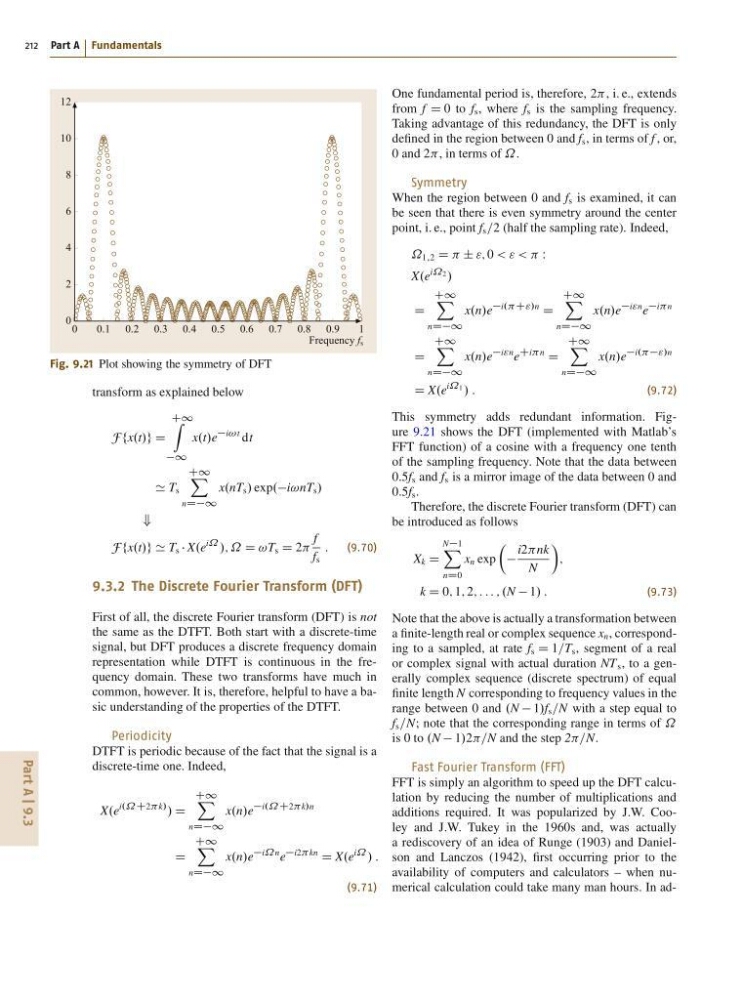
Fig. 9.21 Plot showing the symmetry of DFT
transform as explained below
F fx.t/g D
C1 Z
1
x.t/e
i!t dt
' T s
C1 X
nDD1
x.nT s / exp.i!nT s /
+
F fx.t/g ' T s X.e
i˝
/; ˝ D !T s D 2
f
f s
: (9.70)
9.3.2 The Discrete Fourier Transform (DFT)
First of all, the discrete Fourier transform (DFT) is not
the same as the DTFT. Both start with a discrete-time
signal, but DFT produces a discrete frequency domain
representation while DTFT is continuous in the frequency domain. These two transforms have much in
common, however. It is, therefore, helpful to have a basic understanding of the properties of the DTFT.
Periodicity
DTFT is periodic because of the fact that the signal is a
discrete-time one. Indeed,
X.e
i.˝C2k/
/ D
C1 X
nDD1
x.n/e
i.˝C2k/n
D
C1 X
nDD1
x.n/e
i˝n e
i2kn
D X.e
i˝
/ :
(9.71)
One fundamental period is, therefore, 2, i. e., extends
from f D 0 to f s , where f s is the sampling frequency.
Taking advantage of this redundancy, the DFT is only
defined in the region between 0 and f s , in terms of f , or,
0 and 2, in terms of ˝.
Symmetry
When the region between 0 and f s is examined, it can
be seen that there is even symmetry around the center
point, i. e., point f s =2 (half the sampling rate). Indeed,
˝ 1;2 D ˙ "; 0 < " < < W
X.e
i˝2
/
D
C1 X
nDD1
x.n/e
i..C"/n
D
C1 X
nDD1
x.n/e
i"n e
in
D
C1 X
nDD1
x.n/e
i"n e
Cin
D
C1 X
nDD1
x.n/e
i.."/n
D X.e
i˝1
/ :
(9.72)
This symmetry adds redundant information. Figure 9.21 shows the DFT (implemented with Matlab’s
FFT function) of a cosine with a frequency one tenth
of the sampling frequency. Note that the data between
0.5f s and f s is a mirror image of the data between 0 and
0.5f s .
Therefore, the discrete Fourier transform (DFT) can
be introduced as follows
X k D
N1 X
nD0
x n exp
Â
i2nk
N
Ã
;
k D 0; 1; 2; : : : ; .N 1/ :
(9.73)
Note that the above is actually a transformation between
a finite-length real or complex sequence x n , corresponding to a sampled, at rate f s D 1=T s , segment of a real
or complex signal with actual duration NT s , to a generally complex sequence (discrete spectrum) of equal
finite length N corresponding to frequency values in the
range between 0 and .N 1/f s =N with a step equal to
f s =N; note that the corresponding range in terms of ˝
is 0 to .N 1/2=N and the step 2=N.
Fast Fourier Transform (FFT)
FFT is simply an algorithm to speed up the DFT calculation by reducing the number of multiplications and
additions required. It was popularized by J.W. Cooley and J.W. Tukey in the 1960s and, was actually
a rediscovery of an idea of Runge (1903) and Danielson and Lanczos (1942), first occurring prior to the
availability of computers and calculators – when numerical calculation could take many man hours. In ad-
212 Part A Fundamentals
0
0.1 0.2 0.3 0.4 0.5 0.6 0.7 0.8 0.9
1
Frequency f s
12
10
8
6
4
2
0
Fig. 9.21 Plot showing the symmetry of DFT
transform as explained below
F fx.t/g D
C1 Z
1
x.t/e
i!t dt
' T s
C1 X
nDD1
x.nT s / exp.i!nT s /
+
F fx.t/g ' T s X.e
i˝
/; ˝ D !T s D 2
f
f s
: (9.70)
9.3.2 The Discrete Fourier Transform (DFT)
First of all, the discrete Fourier transform (DFT) is not
the same as the DTFT. Both start with a discrete-time
signal, but DFT produces a discrete frequency domain
representation while DTFT is continuous in the frequency domain. These two transforms have much in
common, however. It is, therefore, helpful to have a basic understanding of the properties of the DTFT.
Periodicity
DTFT is periodic because of the fact that the signal is a
discrete-time one. Indeed,
X.e
i.˝C2k/
/ D
C1 X
nDD1
x.n/e
i.˝C2k/n
D
C1 X
nDD1
x.n/e
i˝n e
i2kn
D X.e
i˝
/ :
(9.71)
One fundamental period is, therefore, 2, i. e., extends
from f D 0 to f s , where f s is the sampling frequency.
Taking advantage of this redundancy, the DFT is only
defined in the region between 0 and f s , in terms of f , or,
0 and 2, in terms of ˝.
Symmetry
When the region between 0 and f s is examined, it can
be seen that there is even symmetry around the center
point, i. e., point f s =2 (half the sampling rate). Indeed,
˝ 1;2 D ˙ "; 0 < " < < W
X.e
i˝2
/
D
C1 X
nDD1
x.n/e
i..C"/n
D
C1 X
nDD1
x.n/e
i"n e
in
D
C1 X
nDD1
x.n/e
i"n e
Cin
D
C1 X
nDD1
x.n/e
i.."/n
D X.e
i˝1
/ :
(9.72)
This symmetry adds redundant information. Figure 9.21 shows the DFT (implemented with Matlab’s
FFT function) of a cosine with a frequency one tenth
of the sampling frequency. Note that the data between
0.5f s and f s is a mirror image of the data between 0 and
0.5f s .
Therefore, the discrete Fourier transform (DFT) can
be introduced as follows
X k D
N1 X
nD0
x n exp
Â
i2nk
N
Ã
;
k D 0; 1; 2; : : : ; .N 1/ :
(9.73)
Note that the above is actually a transformation between
a finite-length real or complex sequence x n , corresponding to a sampled, at rate f s D 1=T s , segment of a real
or complex signal with actual duration NT s , to a generally complex sequence (discrete spectrum) of equal
finite length N corresponding to frequency values in the
range between 0 and .N 1/f s =N with a step equal to
f s =N; note that the corresponding range in terms of ˝
is 0 to .N 1/2=N and the step 2=N.
Fast Fourier Transform (FFT)
FFT is simply an algorithm to speed up the DFT calculation by reducing the number of multiplications and
additions required. It was popularized by J.W. Cooley and J.W. Tukey in the 1960s and, was actually
a rediscovery of an idea of Runge (1903) and Danielson and Lanczos (1942), first occurring prior to the
availability of computers and calculators – when numerical calculation could take many man hours. In ad-