

Part A | 9.2
210 Part A Fundamentals
x (n)
y (n)
z
–1
z
–1
b M
b 0
– a N
z
–1
b 2
– a 2
b 1
– a 1
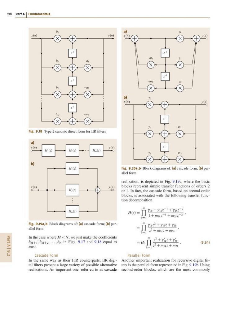
Fig. 9.18 Type 2 canonic direct form for IIR filters
x (n)
x (n)
a)
b)
y (n)
y (n)
H 2 (z)
H m (z)
H 1 (z)
H 2 (z)
H m (z)
H 1 (z)
Fig. 9.19a,b Block diagrams of: (a) cascade form; (b) parallel form
In the case where M < N, we just make the coefficients
b MC1 ; b MC2 ; : : : ; b N in Figs. 9.17 and 9.18 equal to
zero.
Cascade Form
In the same way as their FIR counterparts, IIR digital filters present a large variety of possible alternative
realizations. An important one, referred to as cascade
x (n)
y (n)
z
–1
γ 0
z
–1
γ 2
–m 2
γ 1
–m 1
x (n)
a)
b)
y (n)
z
–1
z
–1
–m 2
–m 1
γ 2
γ 1
γ 0
Fig. 9.20a,b Block diagrams of: (a) cascade form; (b) parallel form
realization, is depicted in Fig. 9.19a, where the basic
blocks represent simple transfer functions of orders 2
or 1. In fact, the cascade form, based on second-order
blocks, is associated with the following transfer function decomposition
H.z/ D
m
Y
kD1
0k C 1k z
1
C 2k z
2
1 C m 1k z 1 C m 2k z 2 ;
D
m
Y
kD1
0k z
2
C 1k z C 2k
z 2 C m 1k z C m 2k
;
D H 0
m
Y
kD1
z
2
C
0
1k z C
0
2k
z 2 C m 1k z C m 2k
:
(9.64)
Parallel Form
Another important realization for recursive digital filters is the parallel form represented in Fig. 9.19b. Using
second-order blocks, which are the most commonly
210 Part A Fundamentals
x (n)
y (n)
z
–1
z
–1
b M
b 0
– a N
z
–1
b 2
– a 2
b 1
– a 1
Fig. 9.18 Type 2 canonic direct form for IIR filters
x (n)
x (n)
a)
b)
y (n)
y (n)
H 2 (z)
H m (z)
H 1 (z)
H 2 (z)
H m (z)
H 1 (z)
Fig. 9.19a,b Block diagrams of: (a) cascade form; (b) parallel form
In the case where M < N, we just make the coefficients
b MC1 ; b MC2 ; : : : ; b N in Figs. 9.17 and 9.18 equal to
zero.
Cascade Form
In the same way as their FIR counterparts, IIR digital filters present a large variety of possible alternative
realizations. An important one, referred to as cascade
x (n)
y (n)
z
–1
γ 0
z
–1
γ 2
–m 2
γ 1
–m 1
x (n)
a)
b)
y (n)
z
–1
z
–1
–m 2
–m 1
γ 2
γ 1
γ 0
Fig. 9.20a,b Block diagrams of: (a) cascade form; (b) parallel form
realization, is depicted in Fig. 9.19a, where the basic
blocks represent simple transfer functions of orders 2
or 1. In fact, the cascade form, based on second-order
blocks, is associated with the following transfer function decomposition
H.z/ D
m
Y
kD1
0k C 1k z
1
C 2k z
2
1 C m 1k z 1 C m 2k z 2 ;
D
m
Y
kD1
0k z
2
C 1k z C 2k
z 2 C m 1k z C m 2k
;
D H 0
m
Y
kD1
z
2
C
0
1k z C
0
2k
z 2 C m 1k z C m 2k
:
(9.64)
Parallel Form
Another important realization for recursive digital filters is the parallel form represented in Fig. 9.19b. Using
second-order blocks, which are the most commonly