

Part A | 9.2
206 Part A Fundamentals
9.2 Digital Filters
In the previous section we studied different ways of
describing discrete-time systems that are linear and
time invariant. It was verified that the Z-transform
greatly simplifies the analysis of discrete-time systems,
especially those initially described by difference equations.
In this section, we study in finer detail several structures used to realize a given transfer function associated
with a specific difference equation through the use of
the Z-transform. The transfer functions considered here
will be of the polynomial form (non-recursive filters,
FIR) and of the rational-polynomial form (recursive filters, IIR). In the non-recursive case we emphasize the
existence of the important subclass of linear-phase filters. Then we introduce some tools to calculate the
digital network transfer function, as well as to analyze
its internal behavior. We also discuss some properties of
generic digital filter structures associated with practical
discrete-time systems.
9.2.1 Important FIR Filter Structures
Non-recursive filters are characterized by a difference
equation in the form
y.n/ D
M
X
lD0
b l x.n l/ ;
(9.53)
where the b l coefficients are directly related to the system impulse response; that is, b l D h.l/. Owing to the
X (z)
x (n)
m j x (n)
a)
b)
z
–1 X (z)
x (n –1)
x (n )
z
–1
m j
x 1 (n)
x 2 (n)
x j (n)
x 1 (n) + x 2 (n) + ... + x j (n)
c)
Fig. 9.8a–c Classic representation of basic elements of
digital filters: (a) delay; (b) multiplier; (c) adder
finite length of their impulse responses, non-recursive
filters are also referred to as finite-duration impulse response (FIR) filters. We can rewrite (9.53) as follows
y.n/ D
M
X
lD0
h.l/x.n l/ :
(9.54)
Applying the Z-transform to the equation above, we end
up with the following input–output relationship
H.z/ D
Y.z/
X.z/
D
M
X
lD0
h.l/z
l
D
M
X
lD0
b l z
l
:
(9.55)
In practical terms, (9.55) can be implemented in
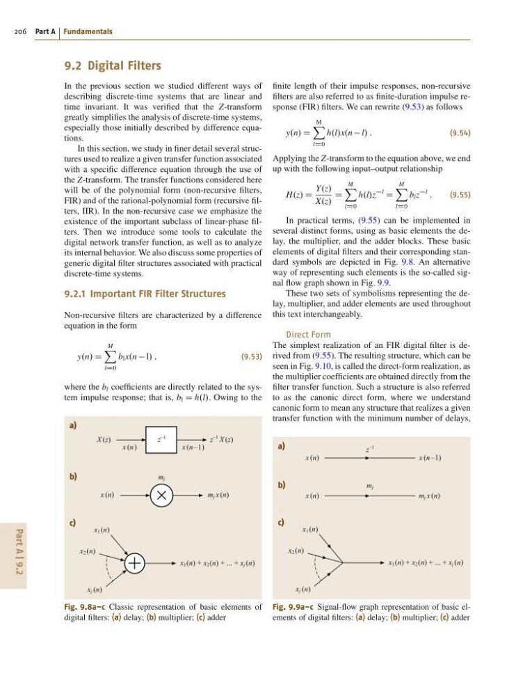
several distinct forms, using as basic elements the delay, the multiplier, and the adder blocks. These basic
elements of digital filters and their corresponding standard symbols are depicted in Fig. 9.8. An alternative
way of representing such elements is the so-called signal flow graph shown in Fig. 9.9.
These two sets of symbolisms representing the delay, multiplier, and adder elements are used throughout
this text interchangeably.
Direct Form
The simplest realization of an FIR digital filter is derived from (9.55). The resulting structure, which can be
seen in Fig. 9.10, is called the direct-form realization, as
the multiplier coefficients are obtained directly from the
filter transfer function. Such a structure is also referred
to as the canonic direct form, where we understand
canonic form to mean any structure that realizes a given
transfer function with the minimum number of delays,
x (n)
x (n)
m j x (n)
a)
b)
x (n –1)
z
–1
m j
x 1 (n)
x 2 (n)
x j (n)
x 1 (n) + x 2 (n) + ... + x j (n)
c)
Fig. 9.9a–c Signal-flow graph representation of basic elements of digital filters: (a) delay; (b) multiplier; (c) adder
206 Part A Fundamentals
9.2 Digital Filters
In the previous section we studied different ways of
describing discrete-time systems that are linear and
time invariant. It was verified that the Z-transform
greatly simplifies the analysis of discrete-time systems,
especially those initially described by difference equations.
In this section, we study in finer detail several structures used to realize a given transfer function associated
with a specific difference equation through the use of
the Z-transform. The transfer functions considered here
will be of the polynomial form (non-recursive filters,
FIR) and of the rational-polynomial form (recursive filters, IIR). In the non-recursive case we emphasize the
existence of the important subclass of linear-phase filters. Then we introduce some tools to calculate the
digital network transfer function, as well as to analyze
its internal behavior. We also discuss some properties of
generic digital filter structures associated with practical
discrete-time systems.
9.2.1 Important FIR Filter Structures
Non-recursive filters are characterized by a difference
equation in the form
y.n/ D
M
X
lD0
b l x.n l/ ;
(9.53)
where the b l coefficients are directly related to the system impulse response; that is, b l D h.l/. Owing to the
X (z)
x (n)
m j x (n)
a)
b)
z
–1 X (z)
x (n –1)
x (n )
z
–1
m j
x 1 (n)
x 2 (n)
x j (n)
x 1 (n) + x 2 (n) + ... + x j (n)
c)
Fig. 9.8a–c Classic representation of basic elements of
digital filters: (a) delay; (b) multiplier; (c) adder
finite length of their impulse responses, non-recursive
filters are also referred to as finite-duration impulse response (FIR) filters. We can rewrite (9.53) as follows
y.n/ D
M
X
lD0
h.l/x.n l/ :
(9.54)
Applying the Z-transform to the equation above, we end
up with the following input–output relationship
H.z/ D
Y.z/
X.z/
D
M
X
lD0
h.l/z
l
D
M
X
lD0
b l z
l
:
(9.55)
In practical terms, (9.55) can be implemented in
several distinct forms, using as basic elements the delay, the multiplier, and the adder blocks. These basic
elements of digital filters and their corresponding standard symbols are depicted in Fig. 9.8. An alternative
way of representing such elements is the so-called signal flow graph shown in Fig. 9.9.
These two sets of symbolisms representing the delay, multiplier, and adder elements are used throughout
this text interchangeably.
Direct Form
The simplest realization of an FIR digital filter is derived from (9.55). The resulting structure, which can be
seen in Fig. 9.10, is called the direct-form realization, as
the multiplier coefficients are obtained directly from the
filter transfer function. Such a structure is also referred
to as the canonic direct form, where we understand
canonic form to mean any structure that realizes a given
transfer function with the minimum number of delays,
x (n)
x (n)
m j x (n)
a)
b)
x (n –1)
z
–1
m j
x 1 (n)
x 2 (n)
x j (n)
x 1 (n) + x 2 (n) + ... + x j (n)
c)
Fig. 9.9a–c Signal-flow graph representation of basic elements of digital filters: (a) delay; (b) multiplier; (c) adder