

Hydromechanics 7.3 Hydrodynamics 159
Part A | 7.3
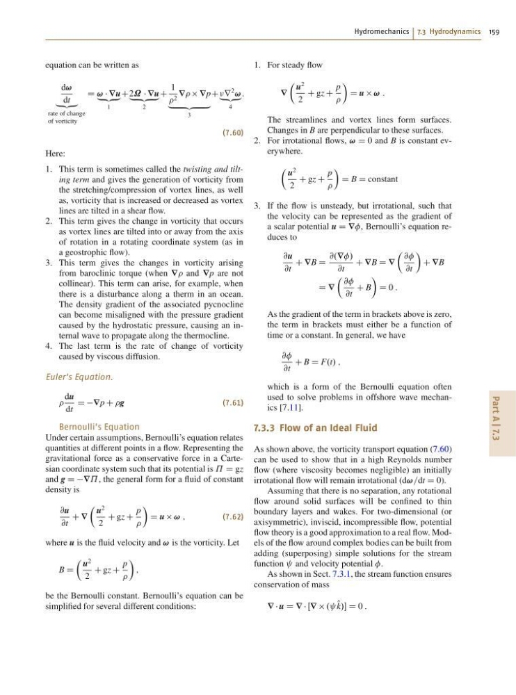
equation can be written as
d!
dt
„ƒ‚…
rate of change
of vorticity
D ! r u
„ƒ‚…
1
C2˝ r u
„ ƒ‚ …
2
C
1
2 r r p
„ ƒ‚ …
3
Cr
2
!
„ƒ‚…
4
:
(7.60)
Here:
1. This term is sometimes called the twisting and tilting term and gives the generation of vorticity from
the stretching/compression of vortex lines, as well
as, vorticity that is increased or decreased as vortex
lines are tilted in a shear flow.
2. This term gives the change in vorticity that occurs
as vortex lines are tilted into or away from the axis
of rotation in a rotating coordinate system (as in
a geostrophic flow).
3. This term gives the changes in vorticity arising
from baroclinic torque (when r and r p are not
collinear). This term can arise, for example, when
there is a disturbance along a therm in an ocean.
The density gradient of the associated pycnocline
can become misaligned with the pressure gradient
caused by the hydrostatic pressure, causing an internal wave to propagate along the thermocline.
4. The last term is the rate of change of vorticity
caused by viscous diffusion.
Euler’s Equation.
du
dt
D Dr p C g
(7.61)
Bernoulli’s Equation
Under certain assumptions, Bernoulli’s equation relates
quantities at different points in a flow. Representing the
gravitational force as a conservative force in a Cartesian coordinate system such that its potential is ˘ D gz
and g D Dr ˘ , the general form for a fluid of constant
density is
@u
@t
C r
 u
2
2
C gz C
p
Ã
D u ! ;
(7.62)
where u is the fluid velocity and ! is the vorticity. Let
B D
 u
2
2
C gz C
p
Ã
;
be the Bernoulli constant. Bernoulli’s equation can be
simplified for several different conditions:
1. For steady flow
r
 u
2
2
C gz C
p
Ã
D u ! :
The streamlines and vortex lines form surfaces.
Changes in B are perpendicular to these surfaces.
2. For irrotational flows, ! D 0 and B is constant everywhere.
 u
2
2
C gz C
p
Ã
D B D constant
3. If the flow is unsteady, but irrotational, such that
the velocity can be represented as the gradient of
a scalar potential u D r , Bernoulli’s equation reduces to
@u
@t
C r B D
@.r /
@t
C r B D r
 @@
@t
Ã
C r B
D r
 @@
@t
C B
Ã
D 0 :
As the gradient of the term in brackets above is zero,
the term in brackets must either be a function of
time or a constant. In general, we have
@@
@t
C B D F.t/ ;
which is a form of the Bernoulli equation often
used to solve problems in offshore wave mechanics [7.11].
7.3.3 Flow of an Ideal Fluid
As shown above, the vorticity transport equation (7.60)
can be used to show that in a high Reynolds number
flow (where viscosity becomes negligible) an initially
irrotational flow will remain irrotational (d!=dt D 0).
Assuming that there is no separation, any rotational
flow around solid surfaces will be confined to thin
boundary layers and wakes. For two-dimensional (or
axisymmetric), inviscid, incompressible flow, potential
flow theory is a good approximation to a real flow. Models of the flow around complex bodies can be built from
adding (superposing) simple solutions for the stream
function and velocity potential .
As shown in Sect. 7.3.1, the stream function ensures
conservation of mass
r u D r Œr . O
k/ D 0 :
Part A | 7.3
equation can be written as
d!
dt
„ƒ‚…
rate of change
of vorticity
D ! r u
„ƒ‚…
1
C2˝ r u
„ ƒ‚ …
2
C
1
2 r r p
„ ƒ‚ …
3
Cr
2
!
„ƒ‚…
4
:
(7.60)
Here:
1. This term is sometimes called the twisting and tilting term and gives the generation of vorticity from
the stretching/compression of vortex lines, as well
as, vorticity that is increased or decreased as vortex
lines are tilted in a shear flow.
2. This term gives the change in vorticity that occurs
as vortex lines are tilted into or away from the axis
of rotation in a rotating coordinate system (as in
a geostrophic flow).
3. This term gives the changes in vorticity arising
from baroclinic torque (when r and r p are not
collinear). This term can arise, for example, when
there is a disturbance along a therm in an ocean.
The density gradient of the associated pycnocline
can become misaligned with the pressure gradient
caused by the hydrostatic pressure, causing an internal wave to propagate along the thermocline.
4. The last term is the rate of change of vorticity
caused by viscous diffusion.
Euler’s Equation.
du
dt
D Dr p C g
(7.61)
Bernoulli’s Equation
Under certain assumptions, Bernoulli’s equation relates
quantities at different points in a flow. Representing the
gravitational force as a conservative force in a Cartesian coordinate system such that its potential is ˘ D gz
and g D Dr ˘ , the general form for a fluid of constant
density is
@u
@t
C r
 u
2
2
C gz C
p
Ã
D u ! ;
(7.62)
where u is the fluid velocity and ! is the vorticity. Let
B D
 u
2
2
C gz C
p
Ã
;
be the Bernoulli constant. Bernoulli’s equation can be
simplified for several different conditions:
1. For steady flow
r
 u
2
2
C gz C
p
Ã
D u ! :
The streamlines and vortex lines form surfaces.
Changes in B are perpendicular to these surfaces.
2. For irrotational flows, ! D 0 and B is constant everywhere.
 u
2
2
C gz C
p
Ã
D B D constant
3. If the flow is unsteady, but irrotational, such that
the velocity can be represented as the gradient of
a scalar potential u D r , Bernoulli’s equation reduces to
@u
@t
C r B D
@.r /
@t
C r B D r
 @@
@t
Ã
C r B
D r
 @@
@t
C B
Ã
D 0 :
As the gradient of the term in brackets above is zero,
the term in brackets must either be a function of
time or a constant. In general, we have
@@
@t
C B D F.t/ ;
which is a form of the Bernoulli equation often
used to solve problems in offshore wave mechanics [7.11].
7.3.3 Flow of an Ideal Fluid
As shown above, the vorticity transport equation (7.60)
can be used to show that in a high Reynolds number
flow (where viscosity becomes negligible) an initially
irrotational flow will remain irrotational (d!=dt D 0).
Assuming that there is no separation, any rotational
flow around solid surfaces will be confined to thin
boundary layers and wakes. For two-dimensional (or
axisymmetric), inviscid, incompressible flow, potential
flow theory is a good approximation to a real flow. Models of the flow around complex bodies can be built from
adding (superposing) simple solutions for the stream
function and velocity potential .
As shown in Sect. 7.3.1, the stream function ensures
conservation of mass
r u D r Œr . O
k/ D 0 :