

Part A | 4.5
88 Part A Fundamentals
and the kinematic free surface boundary condition becomes
2
 @Á
@t
C ı
@Á
@x
@
@x
Ã
D
@
@z
on z D Á :
(4.61)
Rather than using Taylor series about z D 0 to address
the unknown position of the free surface (as was done
for Stokes theory), a power series for the depth dependence is used. This takes advantage of the fact that
vertical variation of dynamical variables is weak in
shallow water
.x; z; t/ D
1
X
nD0
z
h
C 1
Á n n .x; t/ :
(4.62)
This expression for the velocity potential can further be altered to satisfy the governing equation and the
bottom boundary condition. The power series can then
be expressed in terms of 0 , the velocity potential at
z D Dh
D 0
2
2
z
h
C 1
Á 2 @
2
0
@x 2
C
4
24
z
h
C 1
Á 4 @
4
0
@x 4 C O..
6
/ :
(4.63)
This is then substituted into the kinematic and dynamic
free surface boundary conditions and then integrated
over depth. The result is a set of mass and momentum
conservation equations, which are expressed in terms
of powers of and ı, consistent with a weakly dispersive, weakly nonlinear assumption. Retaining terms up
to O.ı; ;
2
/ leads to the Boussinesq equations [4.16]
@Á
@t
C
@
@x
.Œh C Á u/ D 0
(4.64)
@u
@t
C u
@u
@x
C g
@Á
@x
h
2
3
@
3 u
@ 2 x@t
D 0 ;
(4.65)
where u is a depth-averaged velocity.
4.5.1 Properties of Weakly Nonlinear
Shallow Water Waves
The Boussinesq equations can be modeled numerically
for general wave propagation conditions. However, they
can be further transformed into a single wave equation
for Á. This equation is known as the Korteweg–deVries
(KdV) equation
@Á
@t
C c
@Á
@x
C
3c
2h
Á
@Á
@x
C
ch
2
6
@
3
Á
@x 3 D 0 ;
(4.66)
where c D
p
gh. Due to an ambiguity in the derivation
of the KdV equation, there are actually eight formally
identical forms, but the form above is generally the version used.
The KdV equation is, in fact, exactly integrable.
Two general analytic solution forms are possible with
the KdV equation, each representing a wave of permanent form. The first is known as a solitary wave and is
a wave consisting of an isolated hump of water with no
trough. This wave is often used as a proxy for a tsunami
propagating away from its origin. The free surface of
a solitary wave is
Á.x; t/ D Á max sech
2
" p
3
2
Á max
h 3
Á 1=2 .x ct x 0 /
#
;
(4.67)
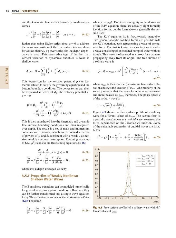
where Á max is the (specified) maximum free surface elevation and x 0 is the location of Á max . One property of the
solitary wave is that the wave form becomes narrower
and more peaked as Á max increases. The phase speed c
of the solitary wave is
c D
p
gh
1 C
Á max
h
Á
:
(4.68)
Figure 4.3 shows the free surface profile of a solitary
wave for different values of Á max . The second form is
a periodic wave known as a cnoidal wave, so named due
to its dependence on the Jacobian cn function. Some
of the calculable properties of cnoidal waves are listed
below
c
2
D gh
Â
1 C
H
h
Ä
1 C
2
m
3E.m/
mK.m/
Ã
; (4.69)
η max = 0.1 m
η max = 0.25 m
η max = 0.5 m
η max = 1 m
–20 –15 –10
–5
0
5
10
15
20
η (m)
x (m)
1
0.9
0.8
0.7
0.6
0.5
0.4
0.3
0.2
0.1
0
Fig. 4.3 Free surface profiles of a solitary wave with different values of Á max
88 Part A Fundamentals
and the kinematic free surface boundary condition becomes
2
 @Á
@t
C ı
@Á
@x
@
@x
Ã
D
@
@z
on z D Á :
(4.61)
Rather than using Taylor series about z D 0 to address
the unknown position of the free surface (as was done
for Stokes theory), a power series for the depth dependence is used. This takes advantage of the fact that
vertical variation of dynamical variables is weak in
shallow water
.x; z; t/ D
1
X
nD0
z
h
C 1
Á n n .x; t/ :
(4.62)
This expression for the velocity potential can further be altered to satisfy the governing equation and the
bottom boundary condition. The power series can then
be expressed in terms of 0 , the velocity potential at
z D Dh
D 0
2
2
z
h
C 1
Á 2 @
2
0
@x 2
C
4
24
z
h
C 1
Á 4 @
4
0
@x 4 C O..
6
/ :
(4.63)
This is then substituted into the kinematic and dynamic
free surface boundary conditions and then integrated
over depth. The result is a set of mass and momentum
conservation equations, which are expressed in terms
of powers of and ı, consistent with a weakly dispersive, weakly nonlinear assumption. Retaining terms up
to O.ı; ;
2
/ leads to the Boussinesq equations [4.16]
@Á
@t
C
@
@x
.Œh C Á u/ D 0
(4.64)
@u
@t
C u
@u
@x
C g
@Á
@x
h
2
3
@
3 u
@ 2 x@t
D 0 ;
(4.65)
where u is a depth-averaged velocity.
4.5.1 Properties of Weakly Nonlinear
Shallow Water Waves
The Boussinesq equations can be modeled numerically
for general wave propagation conditions. However, they
can be further transformed into a single wave equation
for Á. This equation is known as the Korteweg–deVries
(KdV) equation
@Á
@t
C c
@Á
@x
C
3c
2h
Á
@Á
@x
C
ch
2
6
@
3
Á
@x 3 D 0 ;
(4.66)
where c D
p
gh. Due to an ambiguity in the derivation
of the KdV equation, there are actually eight formally
identical forms, but the form above is generally the version used.
The KdV equation is, in fact, exactly integrable.
Two general analytic solution forms are possible with
the KdV equation, each representing a wave of permanent form. The first is known as a solitary wave and is
a wave consisting of an isolated hump of water with no
trough. This wave is often used as a proxy for a tsunami
propagating away from its origin. The free surface of
a solitary wave is
Á.x; t/ D Á max sech
2
" p
3
2
Á max
h 3
Á 1=2 .x ct x 0 /
#
;
(4.67)
where Á max is the (specified) maximum free surface elevation and x 0 is the location of Á max . One property of the
solitary wave is that the wave form becomes narrower
and more peaked as Á max increases. The phase speed c
of the solitary wave is
c D
p
gh
1 C
Á max
h
Á
:
(4.68)
Figure 4.3 shows the free surface profile of a solitary
wave for different values of Á max . The second form is
a periodic wave known as a cnoidal wave, so named due
to its dependence on the Jacobian cn function. Some
of the calculable properties of cnoidal waves are listed
below
c
2
D gh
Â
1 C
H
h
Ä
1 C
2
m
3E.m/
mK.m/
Ã
; (4.69)
η max = 0.1 m
η max = 0.25 m
η max = 0.5 m
η max = 1 m
–20 –15 –10
–5
0
5
10
15
20
η (m)
x (m)
1
0.9
0.8
0.7
0.6
0.5
0.4
0.3
0.2
0.1
0
Fig. 4.3 Free surface profiles of a solitary wave with different values of Á max