

44
Multiscale Hydrologic Remote Sensing: Perspectives and Applications
et al. (2004) inverted Hedges’ dispersion, and Catalán and Haller (2008) achieved
significant results from a wave flume experiment with Kirby’s dispersion. A comparative study of the performance of the inversion of three different wave theories
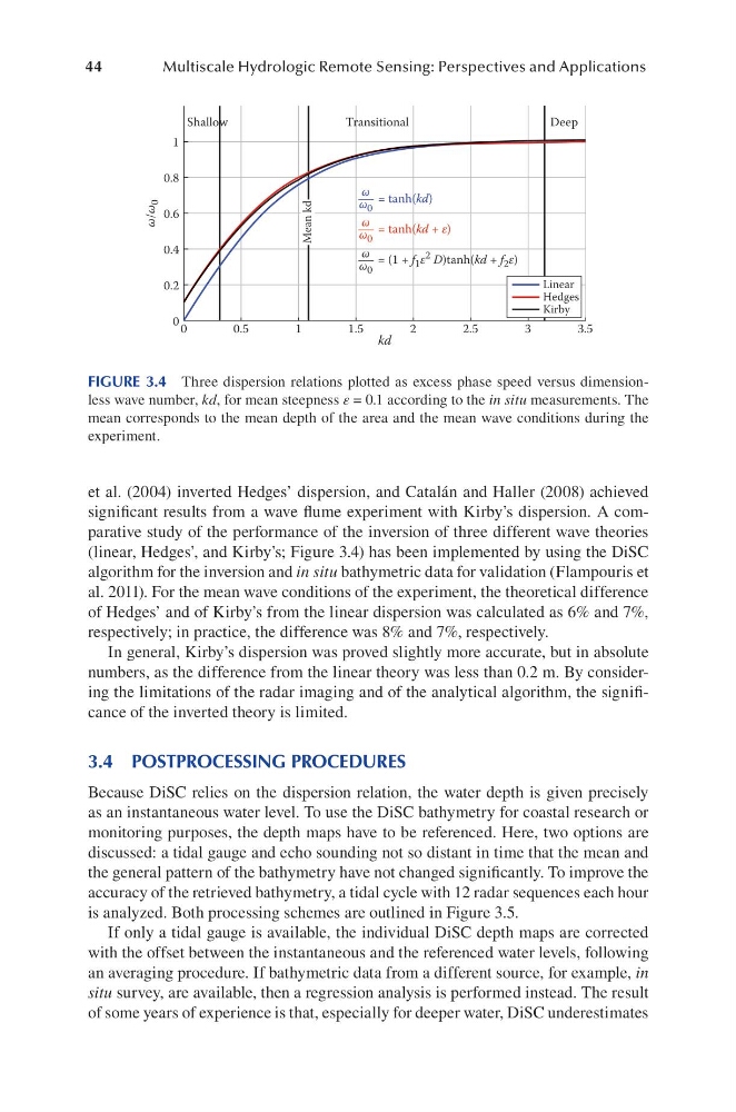
(linear, Hedges’, and Kirby’s; Figure 3.4) has been implemented by using the DiSC
algorithm for the inversion and in situ bathymetric data for validation (Flampouris et
al. 2011). For the mean wave conditions of the experiment, the theoretical difference
of Hedges’ and of Kirby’s from the linear dispersion was calculated as 6% and 7%,
respectively; in practice, the difference was 8% and 7%, respectively.
In general, Kirby’s dispersion was proved slightly more accurate, but in absolute
numbers, as the difference from the linear theory was less than 0.2 m. By considering the limitations of the radar imaging and of the analytical algorithm, the significance of the inverted theory is limited.
3.4 POSTPROCESSING PROCEDURES
Because DiSC relies on the dispersion relation, the water depth is given precisely
as an instantaneous water level. To use the DiSC bathymetry for coastal research or
monitoring purposes, the depth maps have to be referenced. Here, two options are
discussed: a tidal gauge and echo sounding not so distant in time that the mean and
the general pattern of the bathymetry have not changed significantly. To improve the
accuracy of the retrieved bathymetry, a tidal cycle with 12 radar sequences each hour
is analyzed. Both processing schemes are outlined in Figure 3.5.
If only a tidal gauge is available, the individual DiSC depth maps are corrected
with the offset between the instantaneous and the referenced water levels, following
an averaging procedure. If bathymetric data from a different source, for example, in
situ survey, are available, then a regression analysis is performed instead. The result
of some years of experience is that, especially for deeper water, DiSC underestimates
1
0.8
0.6
0.2
0 0
0.5
ω/ω
0
ω
ω 0
ω
ω 0
ω
ω 0
Shallow
Transitional
Deep
1
1.5
2
kd
2.5
3
3.5
Linear
Hedges
Kirby
0.4
— = tanh(kd)
— = tanh(kd + ε)
— = (1 + f 1 ε 2 D)tanh(kd + f 2 ε)
Mean kd
FIGURE 3.4 Three dispersion relations plotted as excess phase speed versus dimensionless wave number, kd, for mean steepness ε = 0.1 according to the in situ measurements. The
mean corresponds to the mean depth of the area and the mean wave conditions during the
experiment.
Multiscale Hydrologic Remote Sensing: Perspectives and Applications
et al. (2004) inverted Hedges’ dispersion, and Catalán and Haller (2008) achieved
significant results from a wave flume experiment with Kirby’s dispersion. A comparative study of the performance of the inversion of three different wave theories
(linear, Hedges’, and Kirby’s; Figure 3.4) has been implemented by using the DiSC
algorithm for the inversion and in situ bathymetric data for validation (Flampouris et
al. 2011). For the mean wave conditions of the experiment, the theoretical difference
of Hedges’ and of Kirby’s from the linear dispersion was calculated as 6% and 7%,
respectively; in practice, the difference was 8% and 7%, respectively.
In general, Kirby’s dispersion was proved slightly more accurate, but in absolute
numbers, as the difference from the linear theory was less than 0.2 m. By considering the limitations of the radar imaging and of the analytical algorithm, the significance of the inverted theory is limited.
3.4 POSTPROCESSING PROCEDURES
Because DiSC relies on the dispersion relation, the water depth is given precisely
as an instantaneous water level. To use the DiSC bathymetry for coastal research or
monitoring purposes, the depth maps have to be referenced. Here, two options are
discussed: a tidal gauge and echo sounding not so distant in time that the mean and
the general pattern of the bathymetry have not changed significantly. To improve the
accuracy of the retrieved bathymetry, a tidal cycle with 12 radar sequences each hour
is analyzed. Both processing schemes are outlined in Figure 3.5.
If only a tidal gauge is available, the individual DiSC depth maps are corrected
with the offset between the instantaneous and the referenced water levels, following
an averaging procedure. If bathymetric data from a different source, for example, in
situ survey, are available, then a regression analysis is performed instead. The result
of some years of experience is that, especially for deeper water, DiSC underestimates
1
0.8
0.6
0.2
0 0
0.5
ω/ω
0
ω
ω 0
ω
ω 0
ω
ω 0
Shallow
Transitional
Deep
1
1.5
2
kd
2.5
3
3.5
Linear
Hedges
Kirby
0.4
— = tanh(kd)
— = tanh(kd + ε)
— = (1 + f 1 ε 2 D)tanh(kd + f 2 ε)
Mean kd
FIGURE 3.4 Three dispersion relations plotted as excess phase speed versus dimensionless wave number, kd, for mean steepness ε = 0.1 according to the in situ measurements. The
mean corresponds to the mean depth of the area and the mean wave conditions during the
experiment.