

485
Validation for Terrestrial Water Storage Variations
river basins shown in Figure 20.1. These river basins are selected because of their
wide coverage across diverse climatic zones in the world. Since all of them have a
basin size larger than 10 6 km 2 , the combined land–atmosphere water balance computation is also applied (Section 20.4.3) to estimate seasonal TWSC, and the obtained
results are compared with GRACE TWS data in Section 20.5.3.
20.3 BACKGROUND
20.3.1 teRReStRial wateR Balance coMPutation
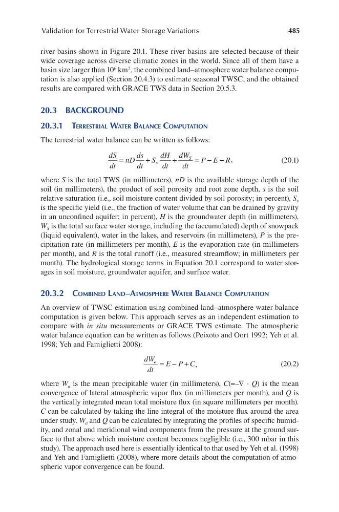
The terrestrial water balance can be written as follows:
dS
dt
nD
ds
dt
S
dH
dt
dW
dt
P E R
y
S
=
+
+
= − − ,
(20.1)
where S is the total TWS (in millimeters), nD is the available storage depth of the
soil (in millimeters), the product of soil porosity and root zone depth, s is the soil
relative saturation (i.e., soil moisture content divided by soil porosity; in percent), S y
is the specific yield (i.e., the fraction of water volume that can be drained by gravity
in an unconfined aquifer; in percent), H is the groundwater depth (in millimeters),
W S is the total surface water storage, including the (accumulated) depth of snowpack
(liquid equivalent), water in the lakes, and reservoirs (in millimeters), P is the precipitation rate (in millimeters per month), E is the evaporation rate (in millimeters
per month), and R is the total runoff (i.e., measured streamflow; in millimeters per
month). The hydrological storage terms in Equation 20.1 correspond to water storages in soil moisture, groundwater aquifer, and surface water.
20.3.2 coMBined land–atMoSPheRe wateR Balance coMPutation
An overview of TWSC estimation using combined land–atmosphere water balance
computation is given below. This approach serves as an independent estimation to
compare with in situ measurements or GRACE TWS estimate. The atmospheric
water balance equation can be written as follows (Peixoto and Oort 1992; Yeh et al.
1998; Yeh and Famiglietti 2008):
dW
dt
E P C
a
= − + ,
(20.2)
where W a is the mean precipitable water (in millimeters), C(=–∇ ⋅ Q) is the mean
convergence of lateral atmospheric vapor flux (in millimeters per month), and Q is
the vertically integrated mean total moisture flux (in square millimeters per month).
C can be calculated by taking the line integral of the moisture flux around the area
under study. W a and Q can be calculated by integrating the profiles of specific humidity, and zonal and meridional wind components from the pressure at the ground surface to that above which moisture content becomes negligible (i.e., 300 mbar in this
study). The approach used here is essentially identical to that used by Yeh et al. (1998)
and Yeh and Famiglietti (2008), where more details about the computation of atmospheric vapor convergence can be found.
Validation for Terrestrial Water Storage Variations
river basins shown in Figure 20.1. These river basins are selected because of their
wide coverage across diverse climatic zones in the world. Since all of them have a
basin size larger than 10 6 km 2 , the combined land–atmosphere water balance computation is also applied (Section 20.4.3) to estimate seasonal TWSC, and the obtained
results are compared with GRACE TWS data in Section 20.5.3.
20.3 BACKGROUND
20.3.1 teRReStRial wateR Balance coMPutation
The terrestrial water balance can be written as follows:
dS
dt
nD
ds
dt
S
dH
dt
dW
dt
P E R
y
S
=
+
+
= − − ,
(20.1)
where S is the total TWS (in millimeters), nD is the available storage depth of the
soil (in millimeters), the product of soil porosity and root zone depth, s is the soil
relative saturation (i.e., soil moisture content divided by soil porosity; in percent), S y
is the specific yield (i.e., the fraction of water volume that can be drained by gravity
in an unconfined aquifer; in percent), H is the groundwater depth (in millimeters),
W S is the total surface water storage, including the (accumulated) depth of snowpack
(liquid equivalent), water in the lakes, and reservoirs (in millimeters), P is the precipitation rate (in millimeters per month), E is the evaporation rate (in millimeters
per month), and R is the total runoff (i.e., measured streamflow; in millimeters per
month). The hydrological storage terms in Equation 20.1 correspond to water storages in soil moisture, groundwater aquifer, and surface water.
20.3.2 coMBined land–atMoSPheRe wateR Balance coMPutation
An overview of TWSC estimation using combined land–atmosphere water balance
computation is given below. This approach serves as an independent estimation to
compare with in situ measurements or GRACE TWS estimate. The atmospheric
water balance equation can be written as follows (Peixoto and Oort 1992; Yeh et al.
1998; Yeh and Famiglietti 2008):
dW
dt
E P C
a
= − + ,
(20.2)
where W a is the mean precipitable water (in millimeters), C(=–∇ ⋅ Q) is the mean
convergence of lateral atmospheric vapor flux (in millimeters per month), and Q is
the vertically integrated mean total moisture flux (in square millimeters per month).
C can be calculated by taking the line integral of the moisture flux around the area
under study. W a and Q can be calculated by integrating the profiles of specific humidity, and zonal and meridional wind components from the pressure at the ground surface to that above which moisture content becomes negligible (i.e., 300 mbar in this
study). The approach used here is essentially identical to that used by Yeh et al. (1998)
and Yeh and Famiglietti (2008), where more details about the computation of atmospheric vapor convergence can be found.