

448
Multiscale Hydrologic Remote Sensing: Perspectives and Applications
application at the global scale in an operational manner; however, they often work
well within a narrow range of surface conditions for which they were developed
and calibrated (e.g., Wood et al. 2003; French et al. 2005; Bastiaanssen et al. 2005;
Courault et al. 2005; Tasumi et al. 2005; McCabe and Wood 2006).
19.2.3 PenMan–Monteith logic
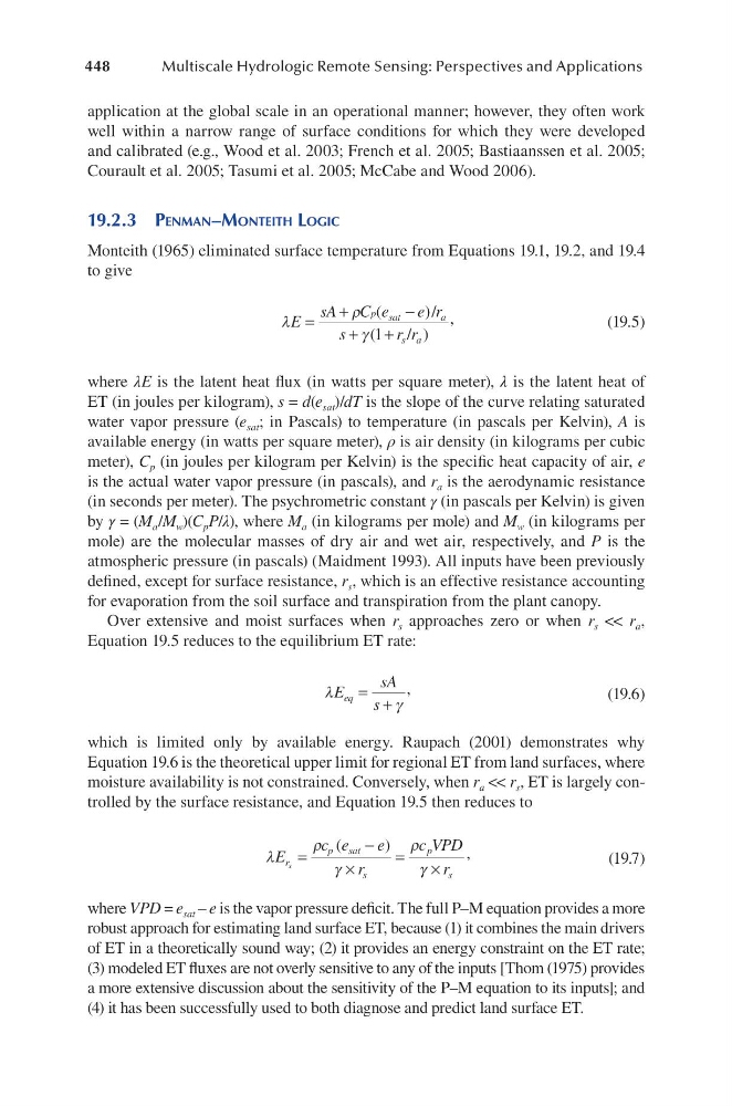
Monteith (1965) eliminated surface temperature from Equations 19.1, 19.2, and 19.4
to give
λ
ρ
γ
E
sA C e
e r
s
r r
p sat
a
s a
=
+
−
+
+
(
)/
(
/ )
1
,
(19.5)
where λE is the latent heat flux (in watts per square meter), λ is the latent heat of
ET (in joules per kilogram), s = d(e sat )/dT is the slope of the curve relating saturated
water vapor pressure (e sat ; in Pascals) to temperature (in pascals per Kelvin), A is
available energy (in watts per square meter), ρ is air density (in kilograms per cubic
meter), C p (in joules per kilogram per Kelvin) is the specific heat capacity of air, e
is the actual water vapor pressure (in pascals), and r a is the aerodynamic resistance
(in seconds per meter). The psychrometric constant γ (in pascals per Kelvin) is given
by γ = (M a /M w )(C p P/λ), where M a (in kilograms per mole) and M w (in kilograms per
mole) are the molecular masses of dry air and wet air, respectively, and P is the
atmospheric pressure (in pascals) (Maidment 1993). All inputs have been previously
defined, except for surface resistance, r s , which is an effective resistance accounting
for evaporation from the soil surface and transpiration from the plant canopy.
Over extensive and moist surfaces when r s approaches zero or when r s << r a ,
Equation 19.5 reduces to the equilibrium ET rate:
λ
γ
E
sA
s
eq = +
,
(19.6)
which is limited only by available energy. Raupach (2001) demonstrates why
Equation 19.6 is the theoretical upper limit for regional ET from land surfaces, where
moisture availability is not constrained. Conversely, when r a << r s , ET is largely controlled by the surface resistance, and Equation 19.5 then reduces to
λ
ρ
γ
ρ
γ
E
c e
e
r
c VPD
r
r
p
sat
s
p
s
s
=
−
×
=
×
(
)
,
(19.7)
where VPD = e sat – e is the vapor pressure deficit. The full P–M equation provides a more
robust approach for estimating land surface ET, because (1) it combines the main drivers
of ET in a theoretically sound way; (2) it provides an energy constraint on the ET rate;
(3) modeled ET fluxes are not overly sensitive to any of the inputs [Thom (1975) provides
a more extensive discussion about the sensitivity of the P–M equation to its inputs]; and
(4) it has been successfully used to both diagnose and predict land surface ET.
Multiscale Hydrologic Remote Sensing: Perspectives and Applications
application at the global scale in an operational manner; however, they often work
well within a narrow range of surface conditions for which they were developed
and calibrated (e.g., Wood et al. 2003; French et al. 2005; Bastiaanssen et al. 2005;
Courault et al. 2005; Tasumi et al. 2005; McCabe and Wood 2006).
19.2.3 PenMan–Monteith logic
Monteith (1965) eliminated surface temperature from Equations 19.1, 19.2, and 19.4
to give
λ
ρ
γ
E
sA C e
e r
s
r r
p sat
a
s a
=
+
−
+
+
(
)/
(
/ )
1
,
(19.5)
where λE is the latent heat flux (in watts per square meter), λ is the latent heat of
ET (in joules per kilogram), s = d(e sat )/dT is the slope of the curve relating saturated
water vapor pressure (e sat ; in Pascals) to temperature (in pascals per Kelvin), A is
available energy (in watts per square meter), ρ is air density (in kilograms per cubic
meter), C p (in joules per kilogram per Kelvin) is the specific heat capacity of air, e
is the actual water vapor pressure (in pascals), and r a is the aerodynamic resistance
(in seconds per meter). The psychrometric constant γ (in pascals per Kelvin) is given
by γ = (M a /M w )(C p P/λ), where M a (in kilograms per mole) and M w (in kilograms per
mole) are the molecular masses of dry air and wet air, respectively, and P is the
atmospheric pressure (in pascals) (Maidment 1993). All inputs have been previously
defined, except for surface resistance, r s , which is an effective resistance accounting
for evaporation from the soil surface and transpiration from the plant canopy.
Over extensive and moist surfaces when r s approaches zero or when r s << r a ,
Equation 19.5 reduces to the equilibrium ET rate:
λ
γ
E
sA
s
eq = +
,
(19.6)
which is limited only by available energy. Raupach (2001) demonstrates why
Equation 19.6 is the theoretical upper limit for regional ET from land surfaces, where
moisture availability is not constrained. Conversely, when r a << r s , ET is largely controlled by the surface resistance, and Equation 19.5 then reduces to
λ
ρ
γ
ρ
γ
E
c e
e
r
c VPD
r
r
p
sat
s
p
s
s
=
−
×
=
×
(
)
,
(19.7)
where VPD = e sat – e is the vapor pressure deficit. The full P–M equation provides a more
robust approach for estimating land surface ET, because (1) it combines the main drivers
of ET in a theoretically sound way; (2) it provides an energy constraint on the ET rate;
(3) modeled ET fluxes are not overly sensitive to any of the inputs [Thom (1975) provides
a more extensive discussion about the sensitivity of the P–M equation to its inputs]; and
(4) it has been successfully used to both diagnose and predict land surface ET.