

446
Multiscale Hydrologic Remote Sensing: Perspectives and Applications
1998a) directly assume there is a linear relationship between LST and ΔT(=T 0 – T a )
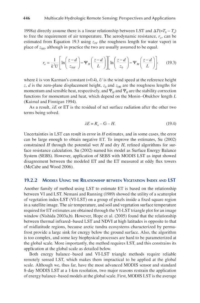
to free the requirement of air temperature. The aerodynamic resistance, r a , can be
estimated from Equation 19.3 using z 0V (the roughness length for water vapor) in
place of z 0H , although in practice the two are usually assumed to be equal.
r k U
z d
z
z d
L
z d
z
a
H
H
=
−
−
−
−
1
2
0
0
ln
ln
Ψ
−
−
Ψ M
z d
L
,
(19.3)
where k is von Karman’s constant (=0.4), U is the wind speed at the reference height
z, d is the zero-plane displacement height, z 0 and z 0H are the roughness lengths for
momentum and sensible heat, respectively, and Ψ M and Ψ H are the stability correction
functions for momentum and heat, which depend on the Monin–Obukhov length L
(Kaimal and Finnigan 1994).
As a result, λE or ET is the residual of net surface radiation after the other two
terms being solved.
λE = R n – G – H.
(19.4)
Uncertainties in LST can result in error in H estimates, and in some cases, the error
can be large enough to obtain negative ET. To improve the estimates, Su (2002)
constrained H through the potential wet H and dry H, refined algorithms for surface resistance calculation. Su (2002) named his model as Surface Energy Balance
System (SEBS). However, application of SEBS with MODIS LST as input showed
disagreement between the modeled ET and the ET measured at eddy flux towers
(McCabe and Wood 2006).
19.2.2 ModelS uSing the RelationShiP Between vegetation index and lSt
Another family of method using LST to estimate ET is based on the relationship
between VI and LST. Nemani and Running (1989) showed the utility of a scatterplot
of vegetation index-LST (VI-LST) on a group of pixels inside a fixed square region
in a satellite image. The air temperature, and soil and vegetation surface temperature
required for ET estimates are obtained through the VI-LST triangle plot for an image
window (Nishida 2003a,b). However, Hope et al. (2005) found that the relationship
between thermal infrared–based LST and NDVI at high latitudes is opposite to that
of midlatitude regions, because arctic tundra ecosystems characterized by permafrost provide a large sink for energy below the ground surface. Also, the algorithm
is too complex, and some key biophysical processes are hard to be parameterized at
the global scale. More importantly, the method requires LST, and this constrains its
application at the global scale as detailed below.
Both energy balance–based and VI-LST triangle methods require reliable
remotely sensed LST, which makes them impractical to be applied at the global
scale. Although we, thus far, have the most advanced MODIS sensor and standard
8-day MODIS LST at a 1-km resolution, two major reasons restrain the application
of energy balance–based models at the global scale. First, MODIS LST is the average
Multiscale Hydrologic Remote Sensing: Perspectives and Applications
1998a) directly assume there is a linear relationship between LST and ΔT(=T 0 – T a )
to free the requirement of air temperature. The aerodynamic resistance, r a , can be
estimated from Equation 19.3 using z 0V (the roughness length for water vapor) in
place of z 0H , although in practice the two are usually assumed to be equal.
r k U
z d
z
z d
L
z d
z
a
H
H
=
−
−
−
−
1
2
0
0
ln
ln
Ψ
−
−
Ψ M
z d
L
,
(19.3)
where k is von Karman’s constant (=0.4), U is the wind speed at the reference height
z, d is the zero-plane displacement height, z 0 and z 0H are the roughness lengths for
momentum and sensible heat, respectively, and Ψ M and Ψ H are the stability correction
functions for momentum and heat, which depend on the Monin–Obukhov length L
(Kaimal and Finnigan 1994).
As a result, λE or ET is the residual of net surface radiation after the other two
terms being solved.
λE = R n – G – H.
(19.4)
Uncertainties in LST can result in error in H estimates, and in some cases, the error
can be large enough to obtain negative ET. To improve the estimates, Su (2002)
constrained H through the potential wet H and dry H, refined algorithms for surface resistance calculation. Su (2002) named his model as Surface Energy Balance
System (SEBS). However, application of SEBS with MODIS LST as input showed
disagreement between the modeled ET and the ET measured at eddy flux towers
(McCabe and Wood 2006).
19.2.2 ModelS uSing the RelationShiP Between vegetation index and lSt
Another family of method using LST to estimate ET is based on the relationship
between VI and LST. Nemani and Running (1989) showed the utility of a scatterplot
of vegetation index-LST (VI-LST) on a group of pixels inside a fixed square region
in a satellite image. The air temperature, and soil and vegetation surface temperature
required for ET estimates are obtained through the VI-LST triangle plot for an image
window (Nishida 2003a,b). However, Hope et al. (2005) found that the relationship
between thermal infrared–based LST and NDVI at high latitudes is opposite to that
of midlatitude regions, because arctic tundra ecosystems characterized by permafrost provide a large sink for energy below the ground surface. Also, the algorithm
is too complex, and some key biophysical processes are hard to be parameterized at
the global scale. More importantly, the method requires LST, and this constrains its
application at the global scale as detailed below.
Both energy balance–based and VI-LST triangle methods require reliable
remotely sensed LST, which makes them impractical to be applied at the global
scale. Although we, thus far, have the most advanced MODIS sensor and standard
8-day MODIS LST at a 1-km resolution, two major reasons restrain the application
of energy balance–based models at the global scale. First, MODIS LST is the average