

423
Microwave Vegetation Indices from Satellite Passive Microwave Sensors
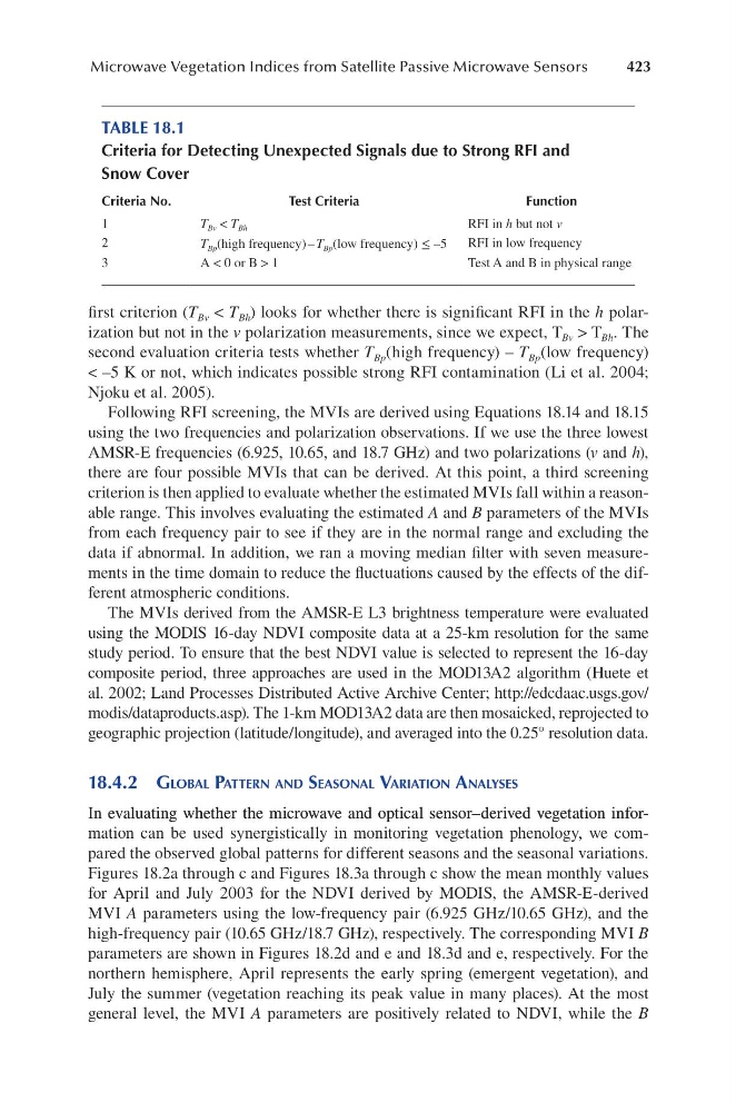
first criterion (T Bv < T Bh ) looks for whether there is significant RFI in the h polarization but not in the v polarization measurements, since we expect, T Bv > T Bh . The
second evaluation criteria tests whether T Bp (high frequency) – T Bp (low frequency)
< –5 K or not, which indicates possible strong RFI contamination (Li et al. 2004;
Njoku et al. 2005).
Following RFI screening, the MVIs are derived using Equations 18.14 and 18.15
using the two frequencies and polarization observations. If we use the three lowest
AMSR-E frequencies (6.925, 10.65, and 18.7 GHz) and two polarizations (v and h),
there are four possible MVIs that can be derived. At this point, a third screening
criterion is then applied to evaluate whether the estimated MVIs fall within a reasonable range. This involves evaluating the estimated A and B parameters of the MVIs
from each frequency pair to see if they are in the normal range and excluding the
data if abnormal. In addition, we ran a moving median filter with seven measurements in the time domain to reduce the fluctuations caused by the effects of the different atmospheric conditions.
The MVIs derived from the AMSR-E L3 brightness temperature were evaluated
using the MODIS 16-day NDVI composite data at a 25-km resolution for the same
study period. To ensure that the best NDVI value is selected to represent the 16-day
composite period, three approaches are used in the MOD13A2 algorithm (Huete et
al. 2002; Land Processes Distributed Active Archive Center; http://edcdaac.usgs .gov/
modis/dataproducts.asp). The 1-km MOD13A2 data are then mosaicked, reprojected to
geographic projection (latitude/longitude), and averaged into the 0.25° resolution data.
18.4.2 gloBal PatteRn and SeaSonal vaRiation analySeS
In evaluating whether the microwave and optical sensor–derived vegetation inforn evaluating whether the microwave and optical sensor–derived vegetation information can be used synergistically in monitoring vegetation phenology, we compared the observed global patterns for different seasons and the seasonal variations.
Figures 18.2a through c and Figures 18.3a through c show the mean monthly values
for April and July 2003 for the NDVI derived by MODIS, the AMSR-E-derived
MVI A parameters using the low-frequency pair (6.925 GHz/10.65 GHz), and the
high-frequency pair (10.65 GHz/18.7 GHz), respectively. The corresponding MVI B
parameters are shown in Figures 18.2d and e and 18.3d and e, respectively. For the
northern hemisphere, April represents the early spring (emergent vegetation), and
July the summer (vegetation reaching its peak value in many places). At the most
general level, the MVI A parameters are positively related to NDVI, while the B
TABLE 18.1
Criteria for Detecting Unexpected Signals due to Strong RFI and
Snow Cover
Criteria No.
Test Criteria
Function
1
T Bv < T Bh
RFI in h but not v
2
T Bp (high frequency) – T Bp (low frequency) ≤ –5
RFI in low frequency
3
A < 0 or B > 1
Test A and B in physical range
Microwave Vegetation Indices from Satellite Passive Microwave Sensors
first criterion (T Bv < T Bh ) looks for whether there is significant RFI in the h polarization but not in the v polarization measurements, since we expect, T Bv > T Bh . The
second evaluation criteria tests whether T Bp (high frequency) – T Bp (low frequency)
< –5 K or not, which indicates possible strong RFI contamination (Li et al. 2004;
Njoku et al. 2005).
Following RFI screening, the MVIs are derived using Equations 18.14 and 18.15
using the two frequencies and polarization observations. If we use the three lowest
AMSR-E frequencies (6.925, 10.65, and 18.7 GHz) and two polarizations (v and h),
there are four possible MVIs that can be derived. At this point, a third screening
criterion is then applied to evaluate whether the estimated MVIs fall within a reasonable range. This involves evaluating the estimated A and B parameters of the MVIs
from each frequency pair to see if they are in the normal range and excluding the
data if abnormal. In addition, we ran a moving median filter with seven measurements in the time domain to reduce the fluctuations caused by the effects of the different atmospheric conditions.
The MVIs derived from the AMSR-E L3 brightness temperature were evaluated
using the MODIS 16-day NDVI composite data at a 25-km resolution for the same
study period. To ensure that the best NDVI value is selected to represent the 16-day
composite period, three approaches are used in the MOD13A2 algorithm (Huete et
al. 2002; Land Processes Distributed Active Archive Center; http://edcdaac.usgs .gov/
modis/dataproducts.asp). The 1-km MOD13A2 data are then mosaicked, reprojected to
geographic projection (latitude/longitude), and averaged into the 0.25° resolution data.
18.4.2 gloBal PatteRn and SeaSonal vaRiation analySeS
In evaluating whether the microwave and optical sensor–derived vegetation inforn evaluating whether the microwave and optical sensor–derived vegetation information can be used synergistically in monitoring vegetation phenology, we compared the observed global patterns for different seasons and the seasonal variations.
Figures 18.2a through c and Figures 18.3a through c show the mean monthly values
for April and July 2003 for the NDVI derived by MODIS, the AMSR-E-derived
MVI A parameters using the low-frequency pair (6.925 GHz/10.65 GHz), and the
high-frequency pair (10.65 GHz/18.7 GHz), respectively. The corresponding MVI B
parameters are shown in Figures 18.2d and e and 18.3d and e, respectively. For the
northern hemisphere, April represents the early spring (emergent vegetation), and
July the summer (vegetation reaching its peak value in many places). At the most
general level, the MVI A parameters are positively related to NDVI, while the B
TABLE 18.1
Criteria for Detecting Unexpected Signals due to Strong RFI and
Snow Cover
Criteria No.
Test Criteria
Function
1
T Bv < T Bh
RFI in h but not v
2
T Bp (high frequency) – T Bp (low frequency) ≤ –5
RFI in low frequency
3
A < 0 or B > 1
Test A and B in physical range