

421
Microwave Vegetation Indices from Satellite Passive Microwave Sensors
fraction cover F v and homogeneity of the surface emissivity properties. For surfaces
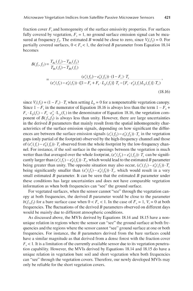
fully covered by vegetation, F v = 1, no ground surface emission signal can be measured at frequency f 2 . The estimated B would be close to zero, since V t ( f 2 ) = 0. For
partially covered surfaces, 0 < F v < 1, the derived B parameter from Equation 18.14
becomes
B f f
T f
T f
T f
T f
f
Bv
Bh
Bv
Bh
v
s
( , )
( )
( )
( )
( )
( (
1 2
2
2
1
1
2
=
−
−
=
ε
) )
( )) (
)
( ( )
( )) ([
−
⋅ −
⋅
−
⋅ − +
ε
ε
ε
h
s
v
s
v
s
h
s
v
f
F T
f
f
F F
2
1
1
1
1
v v
p
s
v
p
v
p
v
L f T F
f L f T
⋅
⋅ −
⋅
⋅
( )]
[
( ) ( )] )
1
1
1
ε
,
(18.16)
since V t ( f 2 ) = (1 – F v ) ∙ T s when setting L p = 0 for a nonpenetrable vegetation canopy.
Since 1 – F v in the numerator of Equation 18.16 is always less than the term 1 – F v +
F v ∙ L p (f 1 ) – F p p
v
v
1
L f
⋅ ⋅
ε
( ) in the denominator of Equation 18.16, the vegetation component of B( f 1 ,f 2 ) is always less than unity. However, there are large uncertainties
in the derived B parameters that mainly result from the spatial inhomogeneity characteristics of the surface emission signals, depending on how significant the differences are between the surface emission signals ( ( )
( ))
ε
ε
v
s
h
s
s
f
f T
2
2
−
⋅ in the vegetation
gaps (only partial of the footprint) observed by the high-frequency channel and those
of ( ( )
( ))
ε
ε
v
s
h
s
s
f
f T
1
1
−
⋅ observed from the whole footprint by the low-frequency channel. For instance, if the soil surface in the openings between the vegetation is much
wetter than that averaged over the whole footprint, ( ( )
( ))
ε
ε
v
s
h
s
s
f
f T
2
2
−
⋅ can be significantly larger than ( ( )
( ))
ε
ε
v
s
h
s
s
f
f T
1
1
−
⋅ , which would lead to the estimated B parameter
being greater than unity. The opposite situation may also occur, ( ( )
( ))
ε
ε
v
s
h
s
s
f
f T
2
2
−
⋅
being significantly smaller than ( ( )
( ))
ε
ε
v
s
h
s
s
f
f T
1
1
−
⋅ , which would result in a very
small estimated B parameter. It can be seen that the estimated B parameter under
these conditions has large uncertainties and does not have comparable vegetation
information as when both frequencies can “see” the ground surface.
For vegetated surfaces, when the sensor cannot “see” through the vegetation canopy at both frequencies, the derived B parameter would be close to the parameter
b(f 1 ,f 2 ) for a bare surface case when 0 < F v < 1. In the case of F v = 1, V t = 0 at both
frequencies. The fluctuations of the derived B parameters observed on different days
would be mainly due to different atmospheric conditions.
As discussed above, the MVIs derived by Equations 18.14 and 18.15 have a nonunique relation in regions where the sensor can “see” the ground surface at both frequencies and the regions where the sensor cannot “see” ground surface at one or both
frequencies. For instance, the B parameters derived from the bare surfaces could
have a similar magnitude as that derived from a dense forest with the fraction cover
F v < 1. It is a limitation of the currently available sensor due to its vegetation penetration capability. However, the MVIs derived by Equations 18.14 and 18.15 do have a
unique relation in vegetation bare soil and short vegetation when both frequencies
can “see” through the vegetation covers. Therefore, our newly developed MVIs may
only be reliable for the short vegetation covers.
Microwave Vegetation Indices from Satellite Passive Microwave Sensors
fraction cover F v and homogeneity of the surface emissivity properties. For surfaces
fully covered by vegetation, F v = 1, no ground surface emission signal can be measured at frequency f 2 . The estimated B would be close to zero, since V t ( f 2 ) = 0. For
partially covered surfaces, 0 < F v < 1, the derived B parameter from Equation 18.14
becomes
B f f
T f
T f
T f
T f
f
Bv
Bh
Bv
Bh
v
s
( , )
( )
( )
( )
( )
( (
1 2
2
2
1
1
2
=
−
−
=
ε
) )
( )) (
)
( ( )
( )) ([
−
⋅ −
⋅
−
⋅ − +
ε
ε
ε
h
s
v
s
v
s
h
s
v
f
F T
f
f
F F
2
1
1
1
1
v v
p
s
v
p
v
p
v
L f T F
f L f T
⋅
⋅ −
⋅
⋅
( )]
[
( ) ( )] )
1
1
1
ε
,
(18.16)
since V t ( f 2 ) = (1 – F v ) ∙ T s when setting L p = 0 for a nonpenetrable vegetation canopy.
Since 1 – F v in the numerator of Equation 18.16 is always less than the term 1 – F v +
F v ∙ L p (f 1 ) – F p p
v
v
1
L f
⋅ ⋅
ε
( ) in the denominator of Equation 18.16, the vegetation component of B( f 1 ,f 2 ) is always less than unity. However, there are large uncertainties
in the derived B parameters that mainly result from the spatial inhomogeneity characteristics of the surface emission signals, depending on how significant the differences are between the surface emission signals ( ( )
( ))
ε
ε
v
s
h
s
s
f
f T
2
2
−
⋅ in the vegetation
gaps (only partial of the footprint) observed by the high-frequency channel and those
of ( ( )
( ))
ε
ε
v
s
h
s
s
f
f T
1
1
−
⋅ observed from the whole footprint by the low-frequency channel. For instance, if the soil surface in the openings between the vegetation is much
wetter than that averaged over the whole footprint, ( ( )
( ))
ε
ε
v
s
h
s
s
f
f T
2
2
−
⋅ can be significantly larger than ( ( )
( ))
ε
ε
v
s
h
s
s
f
f T
1
1
−
⋅ , which would lead to the estimated B parameter
being greater than unity. The opposite situation may also occur, ( ( )
( ))
ε
ε
v
s
h
s
s
f
f T
2
2
−
⋅
being significantly smaller than ( ( )
( ))
ε
ε
v
s
h
s
s
f
f T
1
1
−
⋅ , which would result in a very
small estimated B parameter. It can be seen that the estimated B parameter under
these conditions has large uncertainties and does not have comparable vegetation
information as when both frequencies can “see” the ground surface.
For vegetated surfaces, when the sensor cannot “see” through the vegetation canopy at both frequencies, the derived B parameter would be close to the parameter
b(f 1 ,f 2 ) for a bare surface case when 0 < F v < 1. In the case of F v = 1, V t = 0 at both
frequencies. The fluctuations of the derived B parameters observed on different days
would be mainly due to different atmospheric conditions.
As discussed above, the MVIs derived by Equations 18.14 and 18.15 have a nonunique relation in regions where the sensor can “see” the ground surface at both frequencies and the regions where the sensor cannot “see” ground surface at one or both
frequencies. For instance, the B parameters derived from the bare surfaces could
have a similar magnitude as that derived from a dense forest with the fraction cover
F v < 1. It is a limitation of the currently available sensor due to its vegetation penetration capability. However, the MVIs derived by Equations 18.14 and 18.15 do have a
unique relation in vegetation bare soil and short vegetation when both frequencies
can “see” through the vegetation covers. Therefore, our newly developed MVIs may
only be reliable for the short vegetation covers.