

418
Multiscale Hydrologic Remote Sensing: Perspectives and Applications
using all AIEM simulated surface emissivities are 0.35% and 0.63% for the v and h
polarizations, respectively. For Equation 18.7, they are 0.8% and 1%, respectively.
The relation of bare surface emissivities between two adjacent AMSR-E frequencies as described above is a key discovery that makes it possible to minimize the
effects of the soil surface emission signals when deriving the MVIs that are only
related to vegetation properties.
18.2.3 develoPMent of MicRowave vegetation indiceS
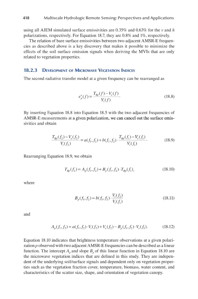
The second radiative transfer model at a given frequency can be rearranged as
ε p
s
Bp
e
t
f
T f V f
V f
( )
( )
( )
( )
=
−
.
(18.8)
By inserting Equation 18.8 into Equation 18.5 with the two adjacent frequencies of
AMSR-E measurements at a given polarization, we can cancel out the surface emisa given polarization, we can cancel out the surface emis, we can cancel out the surface emissivities and obtain
T f
V f
V f
a f f
b f f
T f
Bp
e
t
Bp
( )
( )
( )
( , ) ( , )
( )
2
2
2
1 2
1 2
1
−
=
+
⋅
− V V f
V f
e
t
( )
( )
1
1
.
(18.9)
Rearranging Equation 18.9, we obtain
T f
A f f
B f f T f
Bp
p
p
Bp
( )
( , )
( , )
( )
2
1 2
1 2
1
=
+
⋅
,
(18.10)
where
B f f
b f f
V f
V f
p
t
t
( , )
( , )
( )
( )
1 2
1 2
2
1
=
⋅
(18.11)
and
A f f
a f f V f
V f
B f f V f
p
t
e
p
e
( , )
( , ) ( )
( )
( , ) (
1 2
1 2
2
2
1 2
=
⋅
+
−
⋅
1 1 ).
(18.12)
Equation 18.10 indicates that brightness temperature observations at a given polarization p observed with two adjacent AMSR-E frequencies can be described as a linear
function. The intercept A p and slope B p of this linear function in Equation 18.10 are
the microwave vegetation indices that are defined in this study. They are independent of the underlying soil/surface signals and dependent only on vegetation properties such as the vegetation fraction cover, temperature, biomass, water content, and
characteristics of the scatter size, shape, and orientation of vegetation canopy.
Multiscale Hydrologic Remote Sensing: Perspectives and Applications
using all AIEM simulated surface emissivities are 0.35% and 0.63% for the v and h
polarizations, respectively. For Equation 18.7, they are 0.8% and 1%, respectively.
The relation of bare surface emissivities between two adjacent AMSR-E frequencies as described above is a key discovery that makes it possible to minimize the
effects of the soil surface emission signals when deriving the MVIs that are only
related to vegetation properties.
18.2.3 develoPMent of MicRowave vegetation indiceS
The second radiative transfer model at a given frequency can be rearranged as
ε p
s
Bp
e
t
f
T f V f
V f
( )
( )
( )
( )
=
−
.
(18.8)
By inserting Equation 18.8 into Equation 18.5 with the two adjacent frequencies of
AMSR-E measurements at a given polarization, we can cancel out the surface emisa given polarization, we can cancel out the surface emis, we can cancel out the surface emissivities and obtain
T f
V f
V f
a f f
b f f
T f
Bp
e
t
Bp
( )
( )
( )
( , ) ( , )
( )
2
2
2
1 2
1 2
1
−
=
+
⋅
− V V f
V f
e
t
( )
( )
1
1
.
(18.9)
Rearranging Equation 18.9, we obtain
T f
A f f
B f f T f
Bp
p
p
Bp
( )
( , )
( , )
( )
2
1 2
1 2
1
=
+
⋅
,
(18.10)
where
B f f
b f f
V f
V f
p
t
t
( , )
( , )
( )
( )
1 2
1 2
2
1
=
⋅
(18.11)
and
A f f
a f f V f
V f
B f f V f
p
t
e
p
e
( , )
( , ) ( )
( )
( , ) (
1 2
1 2
2
2
1 2
=
⋅
+
−
⋅
1 1 ).
(18.12)
Equation 18.10 indicates that brightness temperature observations at a given polarization p observed with two adjacent AMSR-E frequencies can be described as a linear
function. The intercept A p and slope B p of this linear function in Equation 18.10 are
the microwave vegetation indices that are defined in this study. They are independent of the underlying soil/surface signals and dependent only on vegetation properties such as the vegetation fraction cover, temperature, biomass, water content, and
characteristics of the scatter size, shape, and orientation of vegetation canopy.