

415
Microwave Vegetation Indices from Satellite Passive Microwave Sensors
T f
F
f T F
f L f R f T F
Bp
v
p
v
v
v
p
v
p
p
e
v
( )
( )
( )
( )
( )
= ⋅
⋅ + ⋅
⋅
⋅
⋅ +
ε
ε
v v
p
s
p
s
v
p
s
s
f L f T
F
f T
⋅
⋅
⋅
+ −
⋅
⋅
ε
ε
( )
( )
(
) ( )
1
,
(18.1)
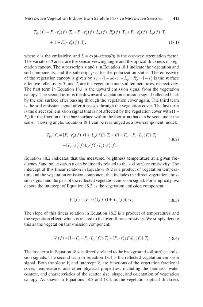
where ε is the emissivity, and L = exp(–τ/cos(θ)) is the one-way attenuation factor.
The variables θ and τ are the sensor viewing angle and the optical thickness of vegetation canopy. The superscripts v and s in Equation 18.1 indicate the vegetation and
soil components, and the subscript p is for the polarization status. The emissivity
of the vegetation canopy is given by ε
ω
p
v
p
L
= − ⋅ −
(
) (
)
1
1
. R p
e
p
s
= −
1 ε is the surface
effective reflectivity. T v and T s are the vegetation and soil temperatures, respectively.
The first term in Equation 18.1 is the upward emission signal from the vegetation
canopy. The second term is the downward vegetation emission signal reflected back
by the soil surface after passing through the vegetation cover again. The third term
is the soil emission signal after it passes through the vegetation cover. The last term
is the direct soil emission signal that is not affected by the vegetation cover with (1 –
F v ) for the fraction of the bare surface within the footprint that can be seen under the
sensor viewing angle. Equation 18.1 can be rearranged as a two-component model:
T f
F
f
L f
T
F F L f
Bp
v
p
v
p
v
v
v
p
( ) [
( ) (
( ))]
([
(
=
⋅
⋅ + ⋅
⋅ + − + ⋅
ε
1
1
) )]
[
( ) ( )] ) ( ).
⋅
−
⋅
⋅ ⋅
T
F
f L f T
f
s
v
p
v
p
v
p
s
ε
ε
(18.2)
Equation 18.2 indicates that the measured brightness temperature at a given freindicates that the measured brightness temperature at a given freindicates that the measured brightness temperature at a given frequency f and polarization p can be linearly related to the soil surface emissivity. The
intercept of this linear relation in Equation 18.2 is a product of vegetation temperature and the vegetation emission component that includes the direct vegetation emission signal and the part of the reflected vegetation emission signal. For simplicity, we
denote the intercept of Equation 18.2 as the vegetation emission component:
V f
F
f
L f
T
e
v
p
v
p
v
( ) [
( ) (
( ))]
=
⋅
⋅ + ⋅
⋅
ε
1
.
(18.3)
The slope of this linear relation in Equation 18.2 is a product of temperatures and
the vegetation effect, which is related to the overall transmissivity. We simply denote
this as the vegetation transmission component:
V f
F F L f T F
f L f T
t
v
v
p
s
v
p
v
p
v
( ) [
( )]
[
( ) ( )]
= − + ⋅
⋅ −
⋅
⋅
1
ε
.
(18.4)
The first term in Equation 18.4 is directly related to the background soil surface emission signals. The second term in Equation 18.4 is the reflected vegetation emission
signal. Both the slope V t and intercept V e are functions of the vegetation fractional
cover, temperature, and other physical properties, including the biomass, water
content, and characteristics of the scatter size, shape, and orientation of vegetation
canopy. As shown in Equations 18.3 and 18.4, as the vegetation optical thickness
Microwave Vegetation Indices from Satellite Passive Microwave Sensors
T f
F
f T F
f L f R f T F
Bp
v
p
v
v
v
p
v
p
p
e
v
( )
( )
( )
( )
( )
= ⋅
⋅ + ⋅
⋅
⋅
⋅ +
ε
ε
v v
p
s
p
s
v
p
s
s
f L f T
F
f T
⋅
⋅
⋅
+ −
⋅
⋅
ε
ε
( )
( )
(
) ( )
1
,
(18.1)
where ε is the emissivity, and L = exp(–τ/cos(θ)) is the one-way attenuation factor.
The variables θ and τ are the sensor viewing angle and the optical thickness of vegetation canopy. The superscripts v and s in Equation 18.1 indicate the vegetation and
soil components, and the subscript p is for the polarization status. The emissivity
of the vegetation canopy is given by ε
ω
p
v
p
L
= − ⋅ −
(
) (
)
1
1
. R p
e
p
s
= −
1 ε is the surface
effective reflectivity. T v and T s are the vegetation and soil temperatures, respectively.
The first term in Equation 18.1 is the upward emission signal from the vegetation
canopy. The second term is the downward vegetation emission signal reflected back
by the soil surface after passing through the vegetation cover again. The third term
is the soil emission signal after it passes through the vegetation cover. The last term
is the direct soil emission signal that is not affected by the vegetation cover with (1 –
F v ) for the fraction of the bare surface within the footprint that can be seen under the
sensor viewing angle. Equation 18.1 can be rearranged as a two-component model:
T f
F
f
L f
T
F F L f
Bp
v
p
v
p
v
v
v
p
( ) [
( ) (
( ))]
([
(
=
⋅
⋅ + ⋅
⋅ + − + ⋅
ε
1
1
) )]
[
( ) ( )] ) ( ).
⋅
−
⋅
⋅ ⋅
T
F
f L f T
f
s
v
p
v
p
v
p
s
ε
ε
(18.2)
Equation 18.2 indicates that the measured brightness temperature at a given freindicates that the measured brightness temperature at a given freindicates that the measured brightness temperature at a given frequency f and polarization p can be linearly related to the soil surface emissivity. The
intercept of this linear relation in Equation 18.2 is a product of vegetation temperature and the vegetation emission component that includes the direct vegetation emission signal and the part of the reflected vegetation emission signal. For simplicity, we
denote the intercept of Equation 18.2 as the vegetation emission component:
V f
F
f
L f
T
e
v
p
v
p
v
( ) [
( ) (
( ))]
=
⋅
⋅ + ⋅
⋅
ε
1
.
(18.3)
The slope of this linear relation in Equation 18.2 is a product of temperatures and
the vegetation effect, which is related to the overall transmissivity. We simply denote
this as the vegetation transmission component:
V f
F F L f T F
f L f T
t
v
v
p
s
v
p
v
p
v
( ) [
( )]
[
( ) ( )]
= − + ⋅
⋅ −
⋅
⋅
1
ε
.
(18.4)
The first term in Equation 18.4 is directly related to the background soil surface emission signals. The second term in Equation 18.4 is the reflected vegetation emission
signal. Both the slope V t and intercept V e are functions of the vegetation fractional
cover, temperature, and other physical properties, including the biomass, water
content, and characteristics of the scatter size, shape, and orientation of vegetation
canopy. As shown in Equations 18.3 and 18.4, as the vegetation optical thickness