

395
Instantaneous Precipitation and Latent Heating Estimation over Land
the computational standpoint if the Jacobians are sparse matrices. This is the case
for the one-dimensional (1-D) Eddington radiative transfer model use by Grecu and
Anagnostou (2002). The derivation of the adjoint for 3-D radiative transfer models
is more complicated, because given their complexity, automatic differentiation procedures are likely to encounter difficulties regarding dependencies among variables.
However, the necessity to develop efficient procedures to evaluate the Jacobian does
not hinder the use of Equation 16.3 with 3-D radiative transfer models.
An efficient procedure for evaluating the Jacobian can be readily developed for
3-D Monte Carlo radiative transfer models. Three-dimensional Monte Carlo radiative transfer models have become increasingly popular in recent years (Davis et al.
2005) and are deemed to be important in the remote sensing of physical variables
that exhibit strong horizontal variability. Precipitation is such variable, and the use
of the 3-D Monte Carlo radiative transfer model in precipitation retrievals is likely to
improve their accuracy. Mathematically, the radiative transfer equation is a Fredholm
integral equation of the second kind that can be iteratively solved (Farnoosh and
Ebrahimi, 2008). Monte Carlo solutions of the radiative transfer equation involve the
evaluation of the associated integrals using statistical methods. That is, any integral
can be interpreted as the expected value of a random variable. Specifically, if f(x)
is the function to be integrated on domain D, one can randomly sample a random
variable in the domain D from an appropriate probability distribution function and
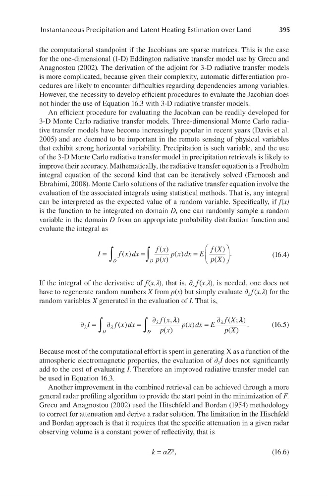
evaluate the integral as
I
f x dx
f x
p x
p x dx E
f X
p X
D
D
=
=
=
∫
∫
( )
( )
( )
( )
( )
( )
.
(16.4)
If the integral of the derivative of f (x,λ), that is, ∂ λ f (x,λ), is needed, one does not
have to regenerate random numbers X from p(x) but simply evaluate ∂ λ f (x,λ) for the
random variables X generated in the evaluation of I. That is,
∂
∂
∂
∂
=
=
=
∫
λ
λ
λ
λ
λ
λ
I
f x dx
f x
p x
p x dx E
f X
p X
D
( )
( , )
( )
( )
( ; )
( )
D D
∫
.
(16.5)
Because most of the computational effort is spent in generating X as a function of the
atmospheric electromagnetic properties, the evaluation of ∂ λ I does not significantly
add to the cost of evaluating I. Therefore an improved radiative transfer model can
be used in Equation 16.3.
Another improvement in the combined retrieval can be achieved through a more
general radar profiling algorithm to provide the start point in the minimization of F.
Grecu and Anagnostou (2002) used the Hitschfeld and Bordan (1954) methodology
to correct for attenuation and derive a radar solution. The limitation in the Hischfeld
and Bordan approach is that it requires that the specific attenuation in a given radar
observing volume is a constant power of reflectivity, that is
k = αZ β ,
(16.6)
Instantaneous Precipitation and Latent Heating Estimation over Land
the computational standpoint if the Jacobians are sparse matrices. This is the case
for the one-dimensional (1-D) Eddington radiative transfer model use by Grecu and
Anagnostou (2002). The derivation of the adjoint for 3-D radiative transfer models
is more complicated, because given their complexity, automatic differentiation procedures are likely to encounter difficulties regarding dependencies among variables.
However, the necessity to develop efficient procedures to evaluate the Jacobian does
not hinder the use of Equation 16.3 with 3-D radiative transfer models.
An efficient procedure for evaluating the Jacobian can be readily developed for
3-D Monte Carlo radiative transfer models. Three-dimensional Monte Carlo radiative transfer models have become increasingly popular in recent years (Davis et al.
2005) and are deemed to be important in the remote sensing of physical variables
that exhibit strong horizontal variability. Precipitation is such variable, and the use
of the 3-D Monte Carlo radiative transfer model in precipitation retrievals is likely to
improve their accuracy. Mathematically, the radiative transfer equation is a Fredholm
integral equation of the second kind that can be iteratively solved (Farnoosh and
Ebrahimi, 2008). Monte Carlo solutions of the radiative transfer equation involve the
evaluation of the associated integrals using statistical methods. That is, any integral
can be interpreted as the expected value of a random variable. Specifically, if f(x)
is the function to be integrated on domain D, one can randomly sample a random
variable in the domain D from an appropriate probability distribution function and
evaluate the integral as
I
f x dx
f x
p x
p x dx E
f X
p X
D
D
=
=
=
∫
∫
( )
( )
( )
( )
( )
( )
.
(16.4)
If the integral of the derivative of f (x,λ), that is, ∂ λ f (x,λ), is needed, one does not
have to regenerate random numbers X from p(x) but simply evaluate ∂ λ f (x,λ) for the
random variables X generated in the evaluation of I. That is,
∂
∂
∂
∂
=
=
=
∫
λ
λ
λ
λ
λ
λ
I
f x dx
f x
p x
p x dx E
f X
p X
D
( )
( , )
( )
( )
( ; )
( )
D D
∫
.
(16.5)
Because most of the computational effort is spent in generating X as a function of the
atmospheric electromagnetic properties, the evaluation of ∂ λ I does not significantly
add to the cost of evaluating I. Therefore an improved radiative transfer model can
be used in Equation 16.3.
Another improvement in the combined retrieval can be achieved through a more
general radar profiling algorithm to provide the start point in the minimization of F.
Grecu and Anagnostou (2002) used the Hitschfeld and Bordan (1954) methodology
to correct for attenuation and derive a radar solution. The limitation in the Hischfeld
and Bordan approach is that it requires that the specific attenuation in a given radar
observing volume is a constant power of reflectivity, that is
k = αZ β ,
(16.6)