

394
Multiscale Hydrologic Remote Sensing: Perspectives and Applications
problem. The function to be minimized is derived from the likelihood of observations conditioned by the set of variables to be retrieved. Specifically, if X is the set
of variables to be retrieved (including two-parameter, i.e., N w , D 0 , representation of
precipitation in each radar observing volume), Z M and T B
M are actual observations,
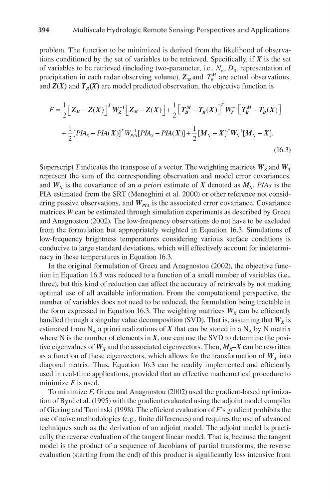
and Z(X) and T B (X) are model predicted observation, the objective function is
F
T
=
−
−
+
−
−
1
2
1
2
1
Z
Z X
W Z
Z X
T
T X
M
M
Z
B
M
B
( )
( )
( )
T T
S
T
PIA
S
PIA PIA
W PIA
W T
T X
X
T
B
M
B
−
−
−
+
−
1
1
1
2
( )
[
( )]
[
− −
+
−
−
−
PIA
T
( )]
[
]
[
].
X
M
X W M
X
X
X
X
1
2
1
(16.3)
Superscript T indicates the transpose of a vector. The weighting matrices W Z and W T
represent the sum of the corresponding observation and model error covariances,
and W X is the covariance of an a priori estimate of X denoted as M X . PIAs is the
PIA estimated from the SRT (Meneghini et al. 2000) or other reference not considering passive observations, and W PIA is the associated error covariance. Covariance
matrices W can be estimated through simulation experiments as described by Grecu
and Anagnostou (2002). The low-frequency observations do not have to be excluded
from the formulation but appropriately weighted in Equation 16.3. Simulations of
low-frequency brightness temperatures considering various surface conditions is
conducive to large standard deviations, which will effectively account for indeterminacy in these temperatures in Equation 16.3.
In the original formulation of Grecu and Anagnostou (2002), the objective function in Equation 16.3 was reduced to a function of a small number of variables (i.e.,
three), but this kind of reduction can affect the accuracy of retrievals by not making
optimal use of all available information. From the computational perspective, the
number of variables does not need to be reduced, the formulation being tractable in
the form expressed in Equation 16.3. The weighting matrices W X can be efficiently
handled through a singular value decomposition (SVD). That is, assuming that W X is
estimated from N A a priori realizations of X that can be stored in a N A by N matrix
where N is the number of elements in X, one can use the SVD to determine the positive eigenvalues of W X and the associated eigenvectors. Then, M X –X can be rewritten
as a function of these eigenvectors, which allows for the transformation of W X into
diagonal matrix. Thus, Equation 16.3 can be readily implemented and efficiently
used in real-time applications, provided that an effective mathematical procedure to
minimize F is used.
To minimize F, Grecu and Anagnostou (2002) used the gradient-based optimization of Byrd et al. (1995) with the gradient evaluated using the adjoint model compiler
of Giering and Taminski (1998). The efficient evaluation of F’s gradient prohibits the
use of naïve methodologies (e.g., finite differences) and requires the use of advanced
techniques such as the derivation of an adjoint model. The adjoint model is practically the reverse evaluation of the tangent linear model. That is, because the tangent
model is the product of a sequence of Jacobians of partial transforms, the reverse
evaluation (starting from the end) of this product is significantly less intensive from
Multiscale Hydrologic Remote Sensing: Perspectives and Applications
problem. The function to be minimized is derived from the likelihood of observations conditioned by the set of variables to be retrieved. Specifically, if X is the set
of variables to be retrieved (including two-parameter, i.e., N w , D 0 , representation of
precipitation in each radar observing volume), Z M and T B
M are actual observations,
and Z(X) and T B (X) are model predicted observation, the objective function is
F
T
=
−
−
+
−
−
1
2
1
2
1
Z
Z X
W Z
Z X
T
T X
M
M
Z
B
M
B
( )
( )
( )
T T
S
T
PIA
S
PIA PIA
W PIA
W T
T X
X
T
B
M
B
−
−
−
+
−
1
1
1
2
( )
[
( )]
[
− −
+
−
−
−
PIA
T
( )]
[
]
[
].
X
M
X W M
X
X
X
X
1
2
1
(16.3)
Superscript T indicates the transpose of a vector. The weighting matrices W Z and W T
represent the sum of the corresponding observation and model error covariances,
and W X is the covariance of an a priori estimate of X denoted as M X . PIAs is the
PIA estimated from the SRT (Meneghini et al. 2000) or other reference not considering passive observations, and W PIA is the associated error covariance. Covariance
matrices W can be estimated through simulation experiments as described by Grecu
and Anagnostou (2002). The low-frequency observations do not have to be excluded
from the formulation but appropriately weighted in Equation 16.3. Simulations of
low-frequency brightness temperatures considering various surface conditions is
conducive to large standard deviations, which will effectively account for indeterminacy in these temperatures in Equation 16.3.
In the original formulation of Grecu and Anagnostou (2002), the objective function in Equation 16.3 was reduced to a function of a small number of variables (i.e.,
three), but this kind of reduction can affect the accuracy of retrievals by not making
optimal use of all available information. From the computational perspective, the
number of variables does not need to be reduced, the formulation being tractable in
the form expressed in Equation 16.3. The weighting matrices W X can be efficiently
handled through a singular value decomposition (SVD). That is, assuming that W X is
estimated from N A a priori realizations of X that can be stored in a N A by N matrix
where N is the number of elements in X, one can use the SVD to determine the positive eigenvalues of W X and the associated eigenvectors. Then, M X –X can be rewritten
as a function of these eigenvectors, which allows for the transformation of W X into
diagonal matrix. Thus, Equation 16.3 can be readily implemented and efficiently
used in real-time applications, provided that an effective mathematical procedure to
minimize F is used.
To minimize F, Grecu and Anagnostou (2002) used the gradient-based optimization of Byrd et al. (1995) with the gradient evaluated using the adjoint model compiler
of Giering and Taminski (1998). The efficient evaluation of F’s gradient prohibits the
use of naïve methodologies (e.g., finite differences) and requires the use of advanced
techniques such as the derivation of an adjoint model. The adjoint model is practically the reverse evaluation of the tangent linear model. That is, because the tangent
model is the product of a sequence of Jacobians of partial transforms, the reverse
evaluation (starting from the end) of this product is significantly less intensive from