

240
Multiscale Hydrologic Remote Sensing: Perspectives and Applications
of the most straightforward ways of applying the GCM output was to combine it
with an observed weather database. This was accomplished by adding the temperature changes to the observed record (e.g., adding the monthly January temperature
increase from a particular scenario to each day of the observed January data, adding
the February increase to the observed February data, and so on) and multiplying the
monthly percentage change in precipitation plus 1 (e.g., 1 + 0.05) by the corresponding month’s observed daily precipitation record. This effectively leaves the historic
variability in the observed record unchanged, except that the temperature data are
shifted by a fixed amount and the precipitation data are scaled. In the present case,
we combined each of the selected GCM scenarios with the daily SNOTEL observations from the basin of interest to generate a 24-year perturbed daily climate. The
SNOTEL observations ran from 1983 through 2006, overlapping almost completely
with the “base period” of the climate simulations.
10.4.7 ReSultS and diScuSSion of SnowMelt Runoff Modeling
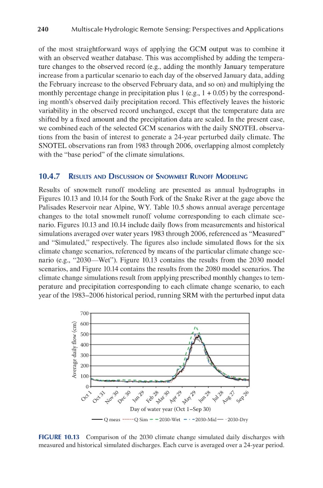
Results of snowmelt runoff modeling are presented as annual hydrographs in
Figures 10.13 and 10.14 for the South Fork of the Snake River at the gage above the
Palisades Reservoir near Alpine, WY. Table 10.5 shows annual average percentage
changes to the total snowmelt runoff volume corresponding to each climate scenario. Figures 10.13 and 10.14 include daily flows from measurements and historical
simulations averaged over water years 1983 through 2006, referenced as “Measured”
and “Simulated,” respectively. The figures also include simulated flows for the six
climate change scenarios, referenced by means of the particular climate change scenario (e.g., “2030—Wet”). Figure 10.13 contains the results from the 2030 model
scenarios, and Figure 10.14 contains the results from the 2080 model scenarios. The
climate change simulations result from applying prescribed monthly changes to temperature and precipitation corresponding to each climate change scenario, to each
year of the 1983–2006 historical period, running SRM with the perturbed input data
700
600
500
400
300
200
100
0
O
c t 1
O
c t 3 1
N
o v 3 0
D
e c 3 0
J a n
2 9
F e b
2 8
M
a r 3 0
A p r 2 9
M
a y 2 9
J u n
2 8
J u l 2 8
A u g
2 7
S e p
2 6
Average daily flow (cm)
Day of water year (Oct 1–Sep 30)
Q meas
Q Sim
2030-Wet
2030-Mid
2030-Dry
FIGURE 10.13 Comparison of the 2030 climate change simulated daily discharges with
measured and historical simulated discharges. Each curve is averaged over a 24-year period.
Multiscale Hydrologic Remote Sensing: Perspectives and Applications
of the most straightforward ways of applying the GCM output was to combine it
with an observed weather database. This was accomplished by adding the temperature changes to the observed record (e.g., adding the monthly January temperature
increase from a particular scenario to each day of the observed January data, adding
the February increase to the observed February data, and so on) and multiplying the
monthly percentage change in precipitation plus 1 (e.g., 1 + 0.05) by the corresponding month’s observed daily precipitation record. This effectively leaves the historic
variability in the observed record unchanged, except that the temperature data are
shifted by a fixed amount and the precipitation data are scaled. In the present case,
we combined each of the selected GCM scenarios with the daily SNOTEL observations from the basin of interest to generate a 24-year perturbed daily climate. The
SNOTEL observations ran from 1983 through 2006, overlapping almost completely
with the “base period” of the climate simulations.
10.4.7 ReSultS and diScuSSion of SnowMelt Runoff Modeling
Results of snowmelt runoff modeling are presented as annual hydrographs in
Figures 10.13 and 10.14 for the South Fork of the Snake River at the gage above the
Palisades Reservoir near Alpine, WY. Table 10.5 shows annual average percentage
changes to the total snowmelt runoff volume corresponding to each climate scenario. Figures 10.13 and 10.14 include daily flows from measurements and historical
simulations averaged over water years 1983 through 2006, referenced as “Measured”
and “Simulated,” respectively. The figures also include simulated flows for the six
climate change scenarios, referenced by means of the particular climate change scenario (e.g., “2030—Wet”). Figure 10.13 contains the results from the 2030 model
scenarios, and Figure 10.14 contains the results from the 2080 model scenarios. The
climate change simulations result from applying prescribed monthly changes to temperature and precipitation corresponding to each climate change scenario, to each
year of the 1983–2006 historical period, running SRM with the perturbed input data
700
600
500
400
300
200
100
0
O
c t 1
O
c t 3 1
N
o v 3 0
D
e c 3 0
J a n
2 9
F e b
2 8
M
a r 3 0
A p r 2 9
M
a y 2 9
J u n
2 8
J u l 2 8
A u g
2 7
S e p
2 6
Average daily flow (cm)
Day of water year (Oct 1–Sep 30)
Q meas
Q Sim
2030-Wet
2030-Mid
2030-Dry
FIGURE 10.13 Comparison of the 2030 climate change simulated daily discharges with
measured and historical simulated discharges. Each curve is averaged over a 24-year period.