

236
Multiscale Hydrologic Remote Sensing: Perspectives and Applications
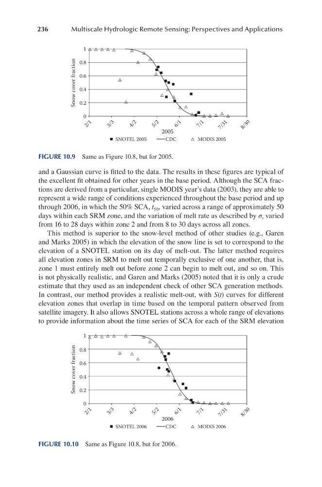
and a Gaussian curve is fitted to the data. The results in these figures are typical of
the excellent fit obtained for other years in the base period. Although the SCA fractions are derived from a particular, single MODIS year’s data (2003), they are able to
represent a wide range of conditions experienced throughout the base period and up
through 2006, in which the 50% SCA, t 50 , varied across a range of approximately 50
days within each SRM zone, and the variation of melt rate as described by σ t varied
from 16 to 28 days within zone 2 and from 8 to 30 days across all zones.
This method is superior to the snow-level method of other studies (e.g., Garen
and Marks 2005) in which the elevation of the snow line is set to correspond to the
elevation of a SNOTEL station on its day of melt-out. The latter method requires
all elevation zones in SRM to melt out temporally exclusive of one another, that is,
zone 1 must entirely melt out before zone 2 can begin to melt out, and so on. This
is not physically realistic, and Garen and Marks (2005) noted that it is only a crude
estimate that they used as an independent check of other SCA generation methods.
In contrast, our method provides a realistic melt-out, with S(t) curves for different
elevation zones that overlap in time based on the temporal pattern observed from
satellite imagery. It also allows SNOTEL stations across a whole range of elevations
to provide information about the time series of SCA for each of the SRM elevation
1
0.8
0.6
0.4
Snow cover fraction
0.2
0
2 / 1
3 / 3
4 / 2
5 / 2
6 / 1
7 / 1
7 / 3 1
8 / 3 0
2005
SNOTEL 2005
CDC
MODIS 2005
FIGURE 10.9 Same as Figure 10.8, but for 2005.
1
0.8
0.6
0.4
Snow cover fraction
0.2
0
2 / 1
3 / 3
4 / 2
5 / 2
6 / 1
7 / 1
7 / 3 1
8 / 3 0
2006
SNOTEL 2006
CDC
MODIS 2006
FIGURE 10.10 Same as Figure 10.8, but for 2006.
Multiscale Hydrologic Remote Sensing: Perspectives and Applications
and a Gaussian curve is fitted to the data. The results in these figures are typical of
the excellent fit obtained for other years in the base period. Although the SCA fractions are derived from a particular, single MODIS year’s data (2003), they are able to
represent a wide range of conditions experienced throughout the base period and up
through 2006, in which the 50% SCA, t 50 , varied across a range of approximately 50
days within each SRM zone, and the variation of melt rate as described by σ t varied
from 16 to 28 days within zone 2 and from 8 to 30 days across all zones.
This method is superior to the snow-level method of other studies (e.g., Garen
and Marks 2005) in which the elevation of the snow line is set to correspond to the
elevation of a SNOTEL station on its day of melt-out. The latter method requires
all elevation zones in SRM to melt out temporally exclusive of one another, that is,
zone 1 must entirely melt out before zone 2 can begin to melt out, and so on. This
is not physically realistic, and Garen and Marks (2005) noted that it is only a crude
estimate that they used as an independent check of other SCA generation methods.
In contrast, our method provides a realistic melt-out, with S(t) curves for different
elevation zones that overlap in time based on the temporal pattern observed from
satellite imagery. It also allows SNOTEL stations across a whole range of elevations
to provide information about the time series of SCA for each of the SRM elevation
1
0.8
0.6
0.4
Snow cover fraction
0.2
0
2 / 1
3 / 3
4 / 2
5 / 2
6 / 1
7 / 1
7 / 3 1
8 / 3 0
2005
SNOTEL 2005
CDC
MODIS 2005
FIGURE 10.9 Same as Figure 10.8, but for 2005.
1
0.8
0.6
0.4
Snow cover fraction
0.2
0
2 / 1
3 / 3
4 / 2
5 / 2
6 / 1
7 / 1
7 / 3 1
8 / 3 0
2006
SNOTEL 2006
CDC
MODIS 2006
FIGURE 10.10 Same as Figure 10.8, but for 2006.