

82
3
Quantification of Early Diagenesis: Dissolved Constituents in Marine Pore Water
rent in the pore water volume of sediments is
bound to the presence of charged ions in
solution, the same deviations are valid (cf. Sect.
2.1.2). The tortuosity (θ) is then calculated by
applying the porosity (φ) to the equation
according to (Berner 1980):
F
⋅
=φ
θ
2
(3.4)
The diffusion coefficient in sediments (D sed ) can
be calculated on the basis of a dimensionless tortuosity and the diffusion coefficient in free solutions of sea-water (D sw in Table 3.1):
2
θ
sw
sed
D
D =
(3.5)
If the tortuosity is not known on account of electric conductivity measurements and the ‘formation
factor’ (F), its value may be estimated, a bit less
accurately, by its empirical relationship to the
porosity. About a dozen different empirical equations are known from literature. The most frequently used is Archie’s Law (Archie 1942):
)
1
(
2
m
−
=φ
θ
(3.6)
The adaptation to specific data is done by means
of (m) as long as parallel values are available for
sediments obtained from direct measurements of
their electrical conductivity. Boudreau (1997)
shows, however, that this relation does not have
any advantage as compared to:
)
(
ln
1
2
2
φ
θ
−
=
(3.7)
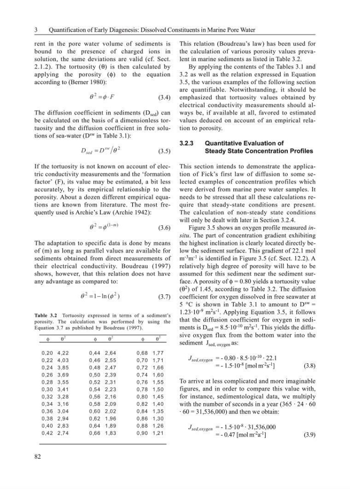
This relation (Boudreau’s law) has been used for
the calculation of various porosity values prevalent in marine sediments as listed in Table 3.2.
By applying the contents of the Tables 3.1 and
3.2 as well as the relation expressed in Equation
3.5, the various examples of the following section
are quantifiable. Notwithstanding, it should be
emphasized that tortuosity values obtained by
electrical conductivity measurements should always be, if available at all, favored to estimated
values deduced on account of an empirical relation to porosity.
3.2.3
Quantitative Evaluation of
Steady State Concentration Profiles
This section intends to demonstrate the application of Fick’s first law of diffusion to some selected examples of concentration profiles which
were derived from marine pore water samples. It
needs to be stressed that all these calculations require that steady-state conditions are present.
The calculation of non-steady state conditions
will only be dealt with later in Section 3.2.4.
Figure 3.5 shows an oxygen profile measured insitu. The part of concentration gradient exhibiting
the highest inclination is clearly located directly below the sediment surface. This gradient of 22.1 mol
m -3 m -1 is identified in Figure 3.5 (cf. Sect. 12.2). A
relatively high degree of porosity will have to be
assumed for this sediment near the sediment surface. A porosity of φ = 0.80 yields a tortuosity value
(θ 2 ) of 1.45, according to Table 3.2. The diffusion
coefficient for oxygen dissolved in free seawater at
5 °C is shown in Table 3.1 to amount to D sw =
1.23·10 -9 m 2 s -1 . Applying Equation 3.5, it follows
that the diffusion coefficient for oxygen in sediments is D sed = 8.5·10 -10 m 2 s -1 . This yields the diffusive oxygen flux from the bottom water into the
sediment J sed, oxygen as:
J sed,oxygen = - 0.80 · 8.5·10 -10 · 22.1
= - 1.5·10 -8 [mol m -2 s -1 ]
(3.8)
To arrive at less complicated and more imaginable
figures, and in order to compare this value with,
for instance, sedimentological data, we multiply
with the number of seconds in a year (365 · 24 · 60
· 60 = 31,536,000) and then we obtain:
J sed,oxygen = - 1.5·10 -8 · 31,536,000
= - 0.47 [mol m -2 a -1 ]
(3.9)
Table 3.2 Tortuosity expressed in terms of a sediment’s
porosity. The calculation was performed by using the
Equation 3.7 as published by Boudreau (1997).
φ
θ
2
φ
θ
2
φ
θ
2
0,20 4,22
0,44 2,64
0,68 1,77
0,22 4,03
0,46 2,55
0,70 1,71
0,24 3,85
0,48 2,47
0,72 1,66
0,26 3,69
0,50 2,39
0,74 1,60
0,28 3,55
0,52 2,31
0,76 1,55
0,30 3,41
0,54 2,23
0,78 1,50
0,32 3,28
0,56 2,16
0,80 1,45
0,34 3,16
0,58 2,09
0,82 1,40
0,36 3,04
0,60 2,02
0,84 1,35
0,38 2,94
0,62 1,96
0,86 1,30
0,40 2,83
0,64 1,89
0,88 1,26
0,42 2,74
0,66 1,83
0,90 1,21
3
Quantification of Early Diagenesis: Dissolved Constituents in Marine Pore Water
rent in the pore water volume of sediments is
bound to the presence of charged ions in
solution, the same deviations are valid (cf. Sect.
2.1.2). The tortuosity (θ) is then calculated by
applying the porosity (φ) to the equation
according to (Berner 1980):
F
⋅
=φ
θ
2
(3.4)
The diffusion coefficient in sediments (D sed ) can
be calculated on the basis of a dimensionless tortuosity and the diffusion coefficient in free solutions of sea-water (D sw in Table 3.1):
2
θ
sw
sed
D
D =
(3.5)
If the tortuosity is not known on account of electric conductivity measurements and the ‘formation
factor’ (F), its value may be estimated, a bit less
accurately, by its empirical relationship to the
porosity. About a dozen different empirical equations are known from literature. The most frequently used is Archie’s Law (Archie 1942):
)
1
(
2
m
−
=φ
θ
(3.6)
The adaptation to specific data is done by means
of (m) as long as parallel values are available for
sediments obtained from direct measurements of
their electrical conductivity. Boudreau (1997)
shows, however, that this relation does not have
any advantage as compared to:
)
(
ln
1
2
2
φ
θ
−
=
(3.7)
This relation (Boudreau’s law) has been used for
the calculation of various porosity values prevalent in marine sediments as listed in Table 3.2.
By applying the contents of the Tables 3.1 and
3.2 as well as the relation expressed in Equation
3.5, the various examples of the following section
are quantifiable. Notwithstanding, it should be
emphasized that tortuosity values obtained by
electrical conductivity measurements should always be, if available at all, favored to estimated
values deduced on account of an empirical relation to porosity.
3.2.3
Quantitative Evaluation of
Steady State Concentration Profiles
This section intends to demonstrate the application of Fick’s first law of diffusion to some selected examples of concentration profiles which
were derived from marine pore water samples. It
needs to be stressed that all these calculations require that steady-state conditions are present.
The calculation of non-steady state conditions
will only be dealt with later in Section 3.2.4.
Figure 3.5 shows an oxygen profile measured insitu. The part of concentration gradient exhibiting
the highest inclination is clearly located directly below the sediment surface. This gradient of 22.1 mol
m -3 m -1 is identified in Figure 3.5 (cf. Sect. 12.2). A
relatively high degree of porosity will have to be
assumed for this sediment near the sediment surface. A porosity of φ = 0.80 yields a tortuosity value
(θ 2 ) of 1.45, according to Table 3.2. The diffusion
coefficient for oxygen dissolved in free seawater at
5 °C is shown in Table 3.1 to amount to D sw =
1.23·10 -9 m 2 s -1 . Applying Equation 3.5, it follows
that the diffusion coefficient for oxygen in sediments is D sed = 8.5·10 -10 m 2 s -1 . This yields the diffusive oxygen flux from the bottom water into the
sediment J sed, oxygen as:
J sed,oxygen = - 0.80 · 8.5·10 -10 · 22.1
= - 1.5·10 -8 [mol m -2 s -1 ]
(3.8)
To arrive at less complicated and more imaginable
figures, and in order to compare this value with,
for instance, sedimentological data, we multiply
with the number of seconds in a year (365 · 24 · 60
· 60 = 31,536,000) and then we obtain:
J sed,oxygen = - 1.5·10 -8 · 31,536,000
= - 0.47 [mol m -2 a -1 ]
(3.9)
Table 3.2 Tortuosity expressed in terms of a sediment’s
porosity. The calculation was performed by using the
Equation 3.7 as published by Boudreau (1997).
φ
θ
2
φ
θ
2
φ
θ
2
0,20 4,22
0,44 2,64
0,68 1,77
0,22 4,03
0,46 2,55
0,70 1,71
0,24 3,85
0,48 2,47
0,72 1,66
0,26 3,69
0,50 2,39
0,74 1,60
0,28 3,55
0,52 2,31
0,76 1,55
0,30 3,41
0,54 2,23
0,78 1,50
0,32 3,28
0,56 2,16
0,80 1,45
0,34 3,16
0,58 2,09
0,82 1,40
0,36 3,04
0,60 2,02
0,84 1,35
0,38 2,94
0,62 1,96
0,86 1,30
0,40 2,83
0,64 1,89
0,88 1,26
0,42 2,74
0,66 1,83
0,90 1,21