

51
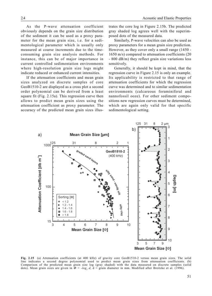
Fig. 2.15 (a) Attenuation coefficients (at 400 kHz) of gravity core GeoB1510-2 versus mean grain sizes. The solid
line indicates a second degree polynomial used to predict mean grain sizes from attenuation coefficients. (b)
Comparison of the predicted mean grain size log (gray shaded) with the data measured on discrete samples (solid
dots). Mean grain sizes are given in Φ = -log 2 d, d = grain diameter in mm. Modified after Breitzke et al. (1996).
As the P-wave attenuation coefficient
obviously depends on the grain size distribution
of the sediment it can be used as a proxy parameter for the mean grain size, i.e. for a sedimentological parameter which is usually only
measured at coarse increments due to the timeconsuming grain size analysis methods. For
instance, this can be of major importance in
current controlled sedimentation environments
where high-resolution grain size logs might
indicate reduced or enhanced current intensities.
If the attenuation coefficients and mean grain
sizes analyzed on discrete samples of core
GeoB1510-2 are displayed as a cross plot a second
order polynomial can be derived from a least
square fit (Fig. 2.15a). This regression curve then
allows to predict mean grain sizes using the
attenuation coefficient as proxy parameter. The
accuracy of the predicted mean grain sizes illustrates the core log in Figure 2.15b. The predicted
gray shaded log agrees well with the superimposed dots of the measured data.
Similarly, P-wave velocities can also be used as
proxy parameters for a mean grain size prediction.
However, as they cover only a small range (1450 -
1650 m/s) compared to attenuation coefficients (20
- 800 dB/m) they reflect grain size variations less
sensitively.
Generally, it should be kept in mind, that the
regression curve in Figure 2.15 is only an example.
Its applicability is restricted to that range of
attenuation coefficients for which the regression
curve was determined and to similar sedimentation
environments (calcareous foraminiferal and
nannofossil ooze). For other sediment compositions new regression curves must be determined,
which are again only valid for that specific
sedimentological setting.
2.4
Acoustic and Elastic Properties
Fig. 2.15 (a) Attenuation coefficients (at 400 kHz) of gravity core GeoB1510-2 versus mean grain sizes. The solid
line indicates a second degree polynomial used to predict mean grain sizes from attenuation coefficients. (b)
Comparison of the predicted mean grain size log (gray shaded) with the data measured on discrete samples (solid
dots). Mean grain sizes are given in Φ = -log 2 d, d = grain diameter in mm. Modified after Breitzke et al. (1996).
As the P-wave attenuation coefficient
obviously depends on the grain size distribution
of the sediment it can be used as a proxy parameter for the mean grain size, i.e. for a sedimentological parameter which is usually only
measured at coarse increments due to the timeconsuming grain size analysis methods. For
instance, this can be of major importance in
current controlled sedimentation environments
where high-resolution grain size logs might
indicate reduced or enhanced current intensities.
If the attenuation coefficients and mean grain
sizes analyzed on discrete samples of core
GeoB1510-2 are displayed as a cross plot a second
order polynomial can be derived from a least
square fit (Fig. 2.15a). This regression curve then
allows to predict mean grain sizes using the
attenuation coefficient as proxy parameter. The
accuracy of the predicted mean grain sizes illustrates the core log in Figure 2.15b. The predicted
gray shaded log agrees well with the superimposed dots of the measured data.
Similarly, P-wave velocities can also be used as
proxy parameters for a mean grain size prediction.
However, as they cover only a small range (1450 -
1650 m/s) compared to attenuation coefficients (20
- 800 dB/m) they reflect grain size variations less
sensitively.
Generally, it should be kept in mind, that the
regression curve in Figure 2.15 is only an example.
Its applicability is restricted to that range of
attenuation coefficients for which the regression
curve was determined and to similar sedimentation
environments (calcareous foraminiferal and
nannofossil ooze). For other sediment compositions new regression curves must be determined,
which are again only valid for that specific
sedimentological setting.
2.4
Acoustic and Elastic Properties