

525
solutions of diagenetic processes. Nevertheless,
these multiple component processes do not constitute a rare exception but represent the normal
case, and must be considered the more one becomes concerned with measuring natural systems.
The solution to this problem consists in the
application of numerical solutions when diagenetic processes are modeled. Such numerical solutions always divide the continuum of reaction
space and reaction time into discrete cells and discrete time intervals. If one divides up the continuum of space and time to a sufficient degree
into discrete cells and time steps (which is not the
decisive problem with the possibilities given by
today’s computers), one will be able to apply
much simpler and better manageable conditions
within the corresponding cells, and with regard to
the expansion of a time interval, so that, in their
entirety, they still will describe a complex system.
Thus, it is possible, for example, to apply the twostep-procedure (Schulz and Reardon 1983), in
which the individual observation of physical
transport (advection, dispersion, diffusion) or any
geochemical multiple component reaction is made
feasible within one interval of time.
15.3.1 Simple Models with Spreadsheet
Software (‘Press-F9-Method’)
Structure of a Worksheet and Oxygen/Nitrate
Modeling
Normal spreadsheet software (e.g. Microsoft -
Excel
®
) present tools especially suited for modeling
stationary and not too complex systems. The wellunderstood decomposition of organic substance
by dissolved oxygen, and the concomitant release
of nitrate, will serve as an example. Nitrate is also
utilized in the oxidation of organic substance in
deeper sections of the diffusion controlled profile.
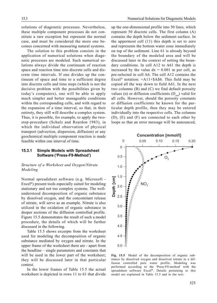
Figure 15.5 demonstrates the result of such a model
procedure, the details of which will be further
discussed in the following.
Table 15.5 shows excerpts from the worksheet
used for modeling the decomposition of organic
substance mediated by oxygen and nitrate. In the
upper frame of the worksheet there are - apart from
the headline – single parameters and constants that
will be used in the lower part of the worksheet;
they will be discussed later in that particular
context.
In the lower frames of Table 15.5 the actual
worksheet is depicted in rows 11 to 61 that divide
up the one-dimensional profile into 50 lines, which
represent 50 discrete cells. The first column (A)
contains the depth below the sediment surface. In
the uppermost cell (11) this depth is set to zero
and represents the bottom water zone immediately
on top of the sediment. Line 61 is already beyond
the boundary of the modeled area and will be
discussed later in the context of setting the boundary conditions. In cell A12 to A61 the depth is
increased by the value dx = 0.001 m per cell, as
pre-selected in cell A6. The cell A12 contains the
Excel
®
notation: =A11+$A$6. This field may be
copied all the way down to field A61. In the next
two columns (B) and (C) we find default porosity
values (n) or diffusion coefficients (D sed ) valid for
all cells. However, should the porosity constants
or diffusion coefficients be known for the particular depth profile, then they may be entered
individually into the respective cells. The columns
(D), (E) and (F) are connected to each other by
loops so that an error message will be announced,
Fig. 15.5 Model of the decomposition of organic substance by dissolved oxygen and dissolved nitrate in a diffusion controlled pore water profile. Modeling was
performed according to the 'Press-F9-method' with the
spreadsheet software Excel ® . Details pertaining to this
model are explained in Table 15.5 and in the text.
15.3
Numerical Solutions for Diagenetic Models
0
0.05
0.10
0.15
0.20
0.5
1.0
1.5
2.0
2.5
3.0
3.5
4.0
4.5
5.0
0
Depth [cm]
Concentration [mmol/l]
O 2
NO 3
-
solutions of diagenetic processes. Nevertheless,
these multiple component processes do not constitute a rare exception but represent the normal
case, and must be considered the more one becomes concerned with measuring natural systems.
The solution to this problem consists in the
application of numerical solutions when diagenetic processes are modeled. Such numerical solutions always divide the continuum of reaction
space and reaction time into discrete cells and discrete time intervals. If one divides up the continuum of space and time to a sufficient degree
into discrete cells and time steps (which is not the
decisive problem with the possibilities given by
today’s computers), one will be able to apply
much simpler and better manageable conditions
within the corresponding cells, and with regard to
the expansion of a time interval, so that, in their
entirety, they still will describe a complex system.
Thus, it is possible, for example, to apply the twostep-procedure (Schulz and Reardon 1983), in
which the individual observation of physical
transport (advection, dispersion, diffusion) or any
geochemical multiple component reaction is made
feasible within one interval of time.
15.3.1 Simple Models with Spreadsheet
Software (‘Press-F9-Method’)
Structure of a Worksheet and Oxygen/Nitrate
Modeling
Normal spreadsheet software (e.g. Microsoft -
Excel
®
) present tools especially suited for modeling
stationary and not too complex systems. The wellunderstood decomposition of organic substance
by dissolved oxygen, and the concomitant release
of nitrate, will serve as an example. Nitrate is also
utilized in the oxidation of organic substance in
deeper sections of the diffusion controlled profile.
Figure 15.5 demonstrates the result of such a model
procedure, the details of which will be further
discussed in the following.
Table 15.5 shows excerpts from the worksheet
used for modeling the decomposition of organic
substance mediated by oxygen and nitrate. In the
upper frame of the worksheet there are - apart from
the headline – single parameters and constants that
will be used in the lower part of the worksheet;
they will be discussed later in that particular
context.
In the lower frames of Table 15.5 the actual
worksheet is depicted in rows 11 to 61 that divide
up the one-dimensional profile into 50 lines, which
represent 50 discrete cells. The first column (A)
contains the depth below the sediment surface. In
the uppermost cell (11) this depth is set to zero
and represents the bottom water zone immediately
on top of the sediment. Line 61 is already beyond
the boundary of the modeled area and will be
discussed later in the context of setting the boundary conditions. In cell A12 to A61 the depth is
increased by the value dx = 0.001 m per cell, as
pre-selected in cell A6. The cell A12 contains the
Excel
®
notation: =A11+$A$6. This field may be
copied all the way down to field A61. In the next
two columns (B) and (C) we find default porosity
values (n) or diffusion coefficients (D sed ) valid for
all cells. However, should the porosity constants
or diffusion coefficients be known for the particular depth profile, then they may be entered
individually into the respective cells. The columns
(D), (E) and (F) are connected to each other by
loops so that an error message will be announced,
Fig. 15.5 Model of the decomposition of organic substance by dissolved oxygen and dissolved nitrate in a diffusion controlled pore water profile. Modeling was
performed according to the 'Press-F9-method' with the
spreadsheet software Excel ® . Details pertaining to this
model are explained in Table 15.5 and in the text.
15.3
Numerical Solutions for Diagenetic Models
0
0.05
0.10
0.15
0.20
0.5
1.0
1.5
2.0
2.5
3.0
3.5
4.0
4.5
5.0
0
Depth [cm]
Concentration [mmol/l]
O 2
NO 3
-