

87
pect this re-oxidation to occur by the action of
dissolved oxygen (cf. Chap. 11).
It is not within the scope of the present discussion to decide whether the variations in the concentration profile that were averaged upon calculating the gradient of 0.0084 mol m -3 m -1 shown in Figure
3.8, merely reflect the inaccuracy pertinent to the
sampling technique and/or the analytical procedure,
or whether they represent discrete processes of their
own. Since they do not vary independently, and
since several points appear to constitute smaller
minima and maxima, it may be suggested that these
measurements do not simply represent analytical
variations, but reasonable and true values. At any
rate, the whole curve leads in its course to very low
values that are reached at a depth of 14 m along with
a distinct change of the gradient’s slope. In many
cases, a precipitation of Mn(II)-carbonate is to be
expected. The identification of such diagenetic
phases anticipated in geochemical modeling is
discussed in more detail in Section 15.1.
3.2.4
The Non-Steady State Situation
and Fick’s Second Law of Diffusion
All examples of the preceding Sections 3.2.2 and
3.2.3 are strictly only valid under steady-state
conditions when concentrations, and hence the
gradients and diffusive fluxes, are constant over
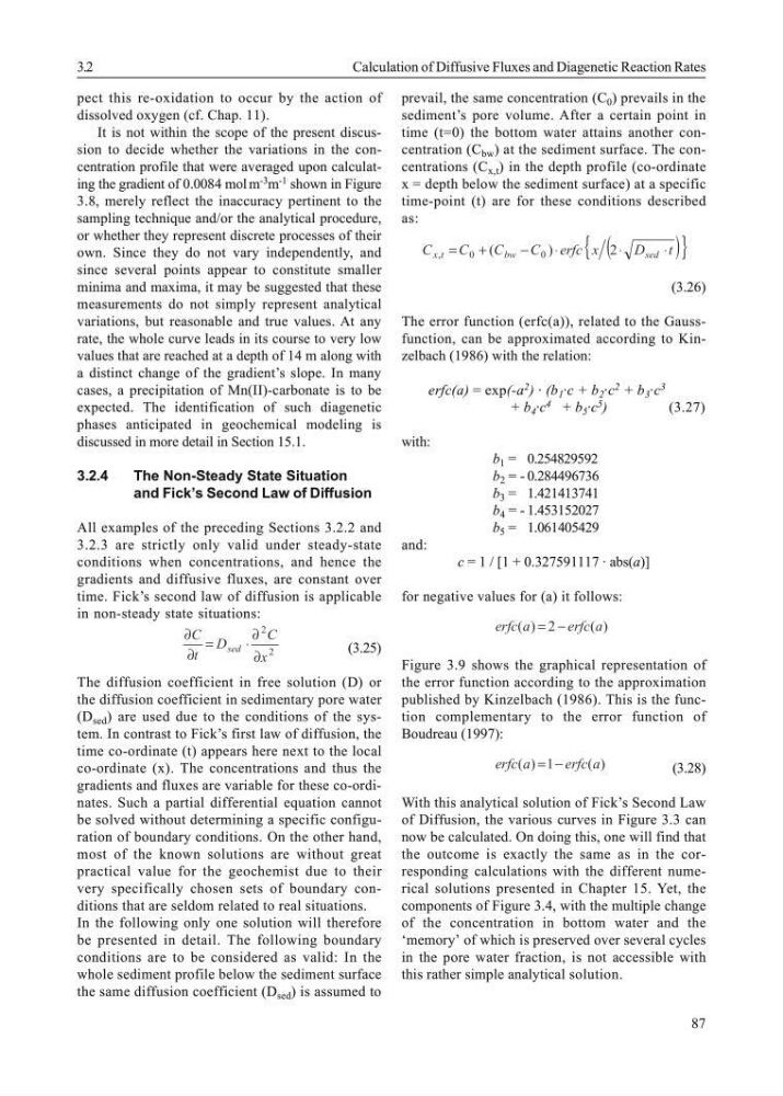
time. Fick’s second law of diffusion is applicable
in non-steady state situations:
(3.25)
The diffusion coefficient in free solution (D) or
the diffusion coefficient in sedimentary pore water
(D sed ) are used due to the conditions of the system. In contrast to Fick’s first law of diffusion, the
time co-ordinate (t) appears here next to the local
co-ordinate (x). The concentrations and thus the
gradients and fluxes are variable for these co-ordinates. Such a partial differential equation cannot
be solved without determining a specific configuration of boundary conditions. On the other hand,
most of the known solutions are without great
practical value for the geochemist due to their
very specifically chosen sets of boundary conditions that are seldom related to real situations.
In the following only one solution will therefore
be presented in detail. The following boundary
conditions are to be considered as valid: In the
whole sediment profile below the sediment surface
the same diffusion coefficient (D sed ) is assumed to
prevail, the same concentration (C 0 ) prevails in the
sediment’s pore volume. After a certain point in
time (t=0) the bottom water attains another concentration (C bw ) at the sediment surface. The concentrations (C x,t ) in the depth profile (co-ordinate
x = depth below the sediment surface) at a specific
time-point (t) are for these conditions described
as:
(
)
{
}
t
D
x
erfc
C
C
C
C
sed
bw
t
x
⋅
⋅
⋅
−
+
=
2
)
(
0
0
,
(3.26)
The error function (erfc(a)), related to the Gaussfunction, can be approximated according to Kinzelbach (1986) with the relation:
erfc(a) = exp(-a 2 ) · (b 1 ·c + b 2 ·c 2 + b 3 ·c 3
+ b 4 ·c 4 + b 5 ·c 5 )
(3.27)
with:
b 1 = 0.254829592
b 2 = - 0.284496736
b 3 = 1.421413741
b 4 = - 1.453152027
b 5 = 1.061405429
and:
c = 1 / [1 + 0.327591117 · abs(a)]
for negative values for (a) it follows:
)
(
2
)
(
a
erfc
a
erfc
−
=
Figure 3.9 shows the graphical representation of
the error function according to the approximation
published by Kinzelbach (1986). This is the function complementary to the error function of
Boudreau (1997):
)
(
1
)
(
a
erfc
a
erfc
−
=
(3.28)
With this analytical solution of Fick’s Second Law
of Diffusion, the various curves in Figure 3.3 can
now be calculated. On doing this, one will find that
the outcome is exactly the same as in the corresponding calculations with the different numerical solutions presented in Chapter 15. Yet, the
components of Figure 3.4, with the multiple change
of the concentration in bottom water and the
‘memory’ of which is preserved over several cycles
in the pore water fraction, is not accessible with
this rather simple analytical solution.
3.2
Calculation of Diffusive Fluxes and Diagenetic Reaction Rates
2
2
x
C
D
t
C
sed ∂
∂
⋅
=
∂
∂
pect this re-oxidation to occur by the action of
dissolved oxygen (cf. Chap. 11).
It is not within the scope of the present discussion to decide whether the variations in the concentration profile that were averaged upon calculating the gradient of 0.0084 mol m -3 m -1 shown in Figure
3.8, merely reflect the inaccuracy pertinent to the
sampling technique and/or the analytical procedure,
or whether they represent discrete processes of their
own. Since they do not vary independently, and
since several points appear to constitute smaller
minima and maxima, it may be suggested that these
measurements do not simply represent analytical
variations, but reasonable and true values. At any
rate, the whole curve leads in its course to very low
values that are reached at a depth of 14 m along with
a distinct change of the gradient’s slope. In many
cases, a precipitation of Mn(II)-carbonate is to be
expected. The identification of such diagenetic
phases anticipated in geochemical modeling is
discussed in more detail in Section 15.1.
3.2.4
The Non-Steady State Situation
and Fick’s Second Law of Diffusion
All examples of the preceding Sections 3.2.2 and
3.2.3 are strictly only valid under steady-state
conditions when concentrations, and hence the
gradients and diffusive fluxes, are constant over
time. Fick’s second law of diffusion is applicable
in non-steady state situations:
(3.25)
The diffusion coefficient in free solution (D) or
the diffusion coefficient in sedimentary pore water
(D sed ) are used due to the conditions of the system. In contrast to Fick’s first law of diffusion, the
time co-ordinate (t) appears here next to the local
co-ordinate (x). The concentrations and thus the
gradients and fluxes are variable for these co-ordinates. Such a partial differential equation cannot
be solved without determining a specific configuration of boundary conditions. On the other hand,
most of the known solutions are without great
practical value for the geochemist due to their
very specifically chosen sets of boundary conditions that are seldom related to real situations.
In the following only one solution will therefore
be presented in detail. The following boundary
conditions are to be considered as valid: In the
whole sediment profile below the sediment surface
the same diffusion coefficient (D sed ) is assumed to
prevail, the same concentration (C 0 ) prevails in the
sediment’s pore volume. After a certain point in
time (t=0) the bottom water attains another concentration (C bw ) at the sediment surface. The concentrations (C x,t ) in the depth profile (co-ordinate
x = depth below the sediment surface) at a specific
time-point (t) are for these conditions described
as:
(
)
{
}
t
D
x
erfc
C
C
C
C
sed
bw
t
x
⋅
⋅
⋅
−
+
=
2
)
(
0
0
,
(3.26)
The error function (erfc(a)), related to the Gaussfunction, can be approximated according to Kinzelbach (1986) with the relation:
erfc(a) = exp(-a 2 ) · (b 1 ·c + b 2 ·c 2 + b 3 ·c 3
+ b 4 ·c 4 + b 5 ·c 5 )
(3.27)
with:
b 1 = 0.254829592
b 2 = - 0.284496736
b 3 = 1.421413741
b 4 = - 1.453152027
b 5 = 1.061405429
and:
c = 1 / [1 + 0.327591117 · abs(a)]
for negative values for (a) it follows:
)
(
2
)
(
a
erfc
a
erfc
−
=
Figure 3.9 shows the graphical representation of
the error function according to the approximation
published by Kinzelbach (1986). This is the function complementary to the error function of
Boudreau (1997):
)
(
1
)
(
a
erfc
a
erfc
−
=
(3.28)
With this analytical solution of Fick’s Second Law
of Diffusion, the various curves in Figure 3.3 can
now be calculated. On doing this, one will find that
the outcome is exactly the same as in the corresponding calculations with the different numerical solutions presented in Chapter 15. Yet, the
components of Figure 3.4, with the multiple change
of the concentration in bottom water and the
‘memory’ of which is preserved over several cycles
in the pore water fraction, is not accessible with
this rather simple analytical solution.
3.2
Calculation of Diffusive Fluxes and Diagenetic Reaction Rates
2
2
x
C
D
t
C
sed ∂
∂
⋅
=
∂
∂