

42
Chapter 3: Climate Spectra and Stochastic Climate Models
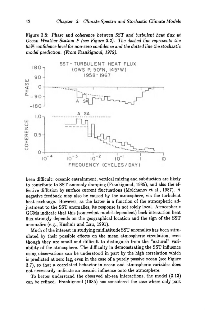
Figure 3.8: Phase and coherence between SST and turbulent heat Bux at
Ocean Weather Station P (see Figure 3.2). The dashed line represents the
95% confidence level tor non-zero confidence and the dotted line the stochastic
model prediction. (From Frankignoul, 1979).
w
180
90
SST· TURBULENT HEAT FLUX
(OWS P, 50 o N, 145°W)
1958- 1967
~
O;---~~_r-------r------_,------_,--__ ~~
r
Cl._ 90
-180
1.0
w
u
Z
w
a: 0 .5
w
r
o
u
A SA
10· 3
10. 2
10. 1
1
10
FREQUENCY (CYCLES/OAYl
been difficult: oceanic entrainment, vertical mixing and subduction are likely
to contribute to SST anomaly damping (Frankignoul, 1985), and also the effective diffusion by surface current fluctuations (Molchanov et al. , 1987). A
negative feedback mayaiso be caused by the atmosphere, via the turbulent
he at exchange. However, as the latter is a function of the atmospheric adjustment to the SST anomalies, its response is not solely local. Atmospheric
GCMs indicate that this (somewhat model-dependent) back inter action heat
flux strongly depends on the geographical location and the sign of the SST
anomalies (e.g., Kushnir and Lau, 1991).
Much of the interest in studying midlatitude SST anomalies has been stimulated by their possible effects on the mean atmospheric circulation, even
though they are small and difficult to distinguish from the "natural" variability of the atmosphere. The difficulty in demonstrating the SST influence
using observations can be understood in part by the high correlation which
is predicted at zero lag, even in the case of a purely passive ocean (see Figure
3.7), so that a correlated behavior in ocean and atmospheric variables does
not necessarily indicate an oceanic influence onto the atmosphere.
To better understand the observed air-sea interactions, the model (3.13)
can be refined. Frankignoul (1985) has considered the case where only part
Chapter 3: Climate Spectra and Stochastic Climate Models
Figure 3.8: Phase and coherence between SST and turbulent heat Bux at
Ocean Weather Station P (see Figure 3.2). The dashed line represents the
95% confidence level tor non-zero confidence and the dotted line the stochastic
model prediction. (From Frankignoul, 1979).
w
180
90
SST· TURBULENT HEAT FLUX
(OWS P, 50 o N, 145°W)
1958- 1967
~
O;---~~_r-------r------_,------_,--__ ~~
r
Cl._ 90
-180
1.0
w
u
Z
w
a: 0 .5
w
r
o
u
A SA
10· 3
10. 2
10. 1
1
10
FREQUENCY (CYCLES/OAYl
been difficult: oceanic entrainment, vertical mixing and subduction are likely
to contribute to SST anomaly damping (Frankignoul, 1985), and also the effective diffusion by surface current fluctuations (Molchanov et al. , 1987). A
negative feedback mayaiso be caused by the atmosphere, via the turbulent
he at exchange. However, as the latter is a function of the atmospheric adjustment to the SST anomalies, its response is not solely local. Atmospheric
GCMs indicate that this (somewhat model-dependent) back inter action heat
flux strongly depends on the geographical location and the sign of the SST
anomalies (e.g., Kushnir and Lau, 1991).
Much of the interest in studying midlatitude SST anomalies has been stimulated by their possible effects on the mean atmospheric circulation, even
though they are small and difficult to distinguish from the "natural" variability of the atmosphere. The difficulty in demonstrating the SST influence
using observations can be understood in part by the high correlation which
is predicted at zero lag, even in the case of a purely passive ocean (see Figure
3.7), so that a correlated behavior in ocean and atmospheric variables does
not necessarily indicate an oceanic influence onto the atmosphere.
To better understand the observed air-sea interactions, the model (3.13)
can be refined. Frankignoul (1985) has considered the case where only part