

Section 3.4: Sea Surface Temperature Anomalies
41
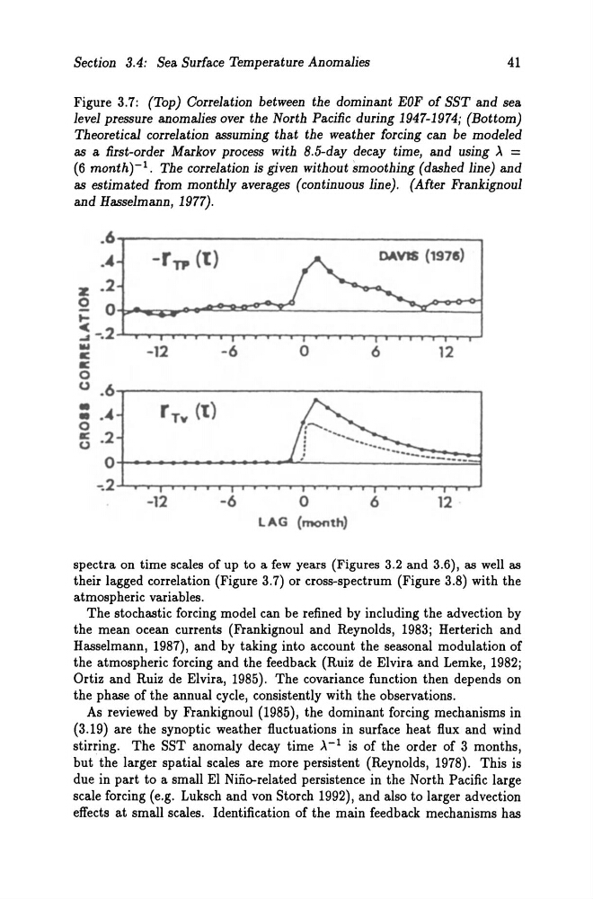
Figure 3.7: (Top) Correlation between the dominant EOF of SST and sea
level press ure anomalies over the North Pacific during 1947-1974; (Bot tom)
Theoretical correlation assuming that the weather forcing can be modeled
as a first-order Markov process with 8.5-day decay time, and using A =
(6 month)-l. The correlation is given without smoothing (dashed line) and
as estimated from monthly averages (continuous line). (After Frankignoul
and Hasselmann, 1977) .
. 6
.4
-r TP (I)
DAVIS (1971)
z .2
0
0
~
~ -.2
.. -12 -6 0 6 12
c
c
0
u .6
• ..4
r Tv (t)
• 0 c .2
u
0
~2
-12
-6
0
6
12
LAG (month)
spectra on time scales of up to a few years (Figures 3.2 and 3.6), as weH as
their lagged correlation (Figure 3.7) or cross-spectrum (Figure 3.8) with the
atmospheric variables.
The stochastic forcing model can be refined by induding the advection by
the mean ocean currents (Frankignoul and Reynolds, 1983; Herterich and
Hasselmann, 1987), and by taking into ac count the seasonal modulation of
the atmospheric forcing and the feedback (Ruiz de Elvira and Lemke, 1982;
Ortiz and Ruiz de Elvira, 1985). The covariance function then depends on
the phase of the annual cyde, consistently with the observations.
As reviewed by Frankignoul (1985), the dominant forcing mechanisms in
(3.19) are the synoptic weather fluctuations in surface heat flux and wind
stirring. The SST anomaly decay time A- 1 is of the order of 3 months,
but the larger spatial scales are more persistent (Reynolds, 1978). This is
due in part to a small EI Nifio-related persistence in the North Pacific large
scale forcing (e.g. Luksch and von Storch 1992), and also to larger advection
effects at small scales. Identification of the main feedback mechanisms has
41
Figure 3.7: (Top) Correlation between the dominant EOF of SST and sea
level press ure anomalies over the North Pacific during 1947-1974; (Bot tom)
Theoretical correlation assuming that the weather forcing can be modeled
as a first-order Markov process with 8.5-day decay time, and using A =
(6 month)-l. The correlation is given without smoothing (dashed line) and
as estimated from monthly averages (continuous line). (After Frankignoul
and Hasselmann, 1977) .
. 6
.4
-r TP (I)
DAVIS (1971)
z .2
0
0
~
~ -.2
.. -12 -6 0 6 12
c
c
0
u .6
• ..4
r Tv (t)
• 0 c .2
u
0
~2
-12
-6
0
6
12
LAG (month)
spectra on time scales of up to a few years (Figures 3.2 and 3.6), as weH as
their lagged correlation (Figure 3.7) or cross-spectrum (Figure 3.8) with the
atmospheric variables.
The stochastic forcing model can be refined by induding the advection by
the mean ocean currents (Frankignoul and Reynolds, 1983; Herterich and
Hasselmann, 1987), and by taking into ac count the seasonal modulation of
the atmospheric forcing and the feedback (Ruiz de Elvira and Lemke, 1982;
Ortiz and Ruiz de Elvira, 1985). The covariance function then depends on
the phase of the annual cyde, consistently with the observations.
As reviewed by Frankignoul (1985), the dominant forcing mechanisms in
(3.19) are the synoptic weather fluctuations in surface heat flux and wind
stirring. The SST anomaly decay time A- 1 is of the order of 3 months,
but the larger spatial scales are more persistent (Reynolds, 1978). This is
due in part to a small EI Nifio-related persistence in the North Pacific large
scale forcing (e.g. Luksch and von Storch 1992), and also to larger advection
effects at small scales. Identification of the main feedback mechanisms has