

38
Chapter 3: Climate Spectra and Stochastic Climate Models
r~(/) = r~ (I)
')
12 '
(3.9)
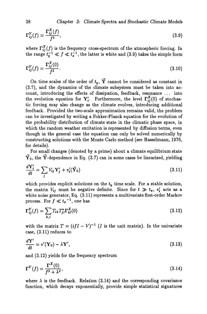
where q; (I) is the frequency cross-spectrum of the atmospheric forcing. In
the range t;l ~ 1 ~ t;l, the latter is white and (3.9) takes the simple form
r~(/) = r~ (0)
')
j2.
(3.10)
On time scales of the order of ty , V cannot be considered as constant in
(3.7), and the dynamics of the climate subsystem must be taken into account, introducing the effects of dissipation, feedback, resonance ... into
the evolution equation for Y~. Furthermore, the level r~(O) of stochastic forcing mayaiso change as the climate evolves, introducing additional
feedback. Provided the two-scale approximation remains valid, the problem
can be investigated by writing a Fokker-Planck equation for the evolution of
the prob ability distribution of climate state in the climatic phase space, in
which the random weather excitation is represented by diffusion terms, even
though in the general case the equation can only be solved numerically by
constructing solutions with the Monte Carlo method (see Hasselmann, 1976,
for details).
For small changes (denoted by a prime) about a climate equilibrium state
Va, the V-dependence in Eq. (3.7) can in some cases be linearized, yielding
(3.11)
which provides explicit solutions on the t y time scale. For a stable solution,
the matrix Vij must be negative definite. Since for t ~ t lll , v~ acts as a
white noise generator, Eq. (3.11) represents a multivariate first-order Markov
process. For 1 ~ t lll -1, one has
r~(I) = I:1h1j*lr:;(0)
(3.12)
k,l
with the matrix T = (ilI - V)-l (I is the unit matrix). In the univariate
case, (3.11) reduces to
d!/ = v/(Y a ) _ >'Y/,
and (3.12) yields for the frequency spectrum
rY (I) = r
X
(0)
j2 + >.2'
(3.13)
(3.14)
where >. is the feedback. Relation (3.14) and the corresponding covariance
function, which decays exponentially, provide simple statistical signatures
Chapter 3: Climate Spectra and Stochastic Climate Models
r~(/) = r~ (I)
')
12 '
(3.9)
where q; (I) is the frequency cross-spectrum of the atmospheric forcing. In
the range t;l ~ 1 ~ t;l, the latter is white and (3.9) takes the simple form
r~(/) = r~ (0)
')
j2.
(3.10)
On time scales of the order of ty , V cannot be considered as constant in
(3.7), and the dynamics of the climate subsystem must be taken into account, introducing the effects of dissipation, feedback, resonance ... into
the evolution equation for Y~. Furthermore, the level r~(O) of stochastic forcing mayaiso change as the climate evolves, introducing additional
feedback. Provided the two-scale approximation remains valid, the problem
can be investigated by writing a Fokker-Planck equation for the evolution of
the prob ability distribution of climate state in the climatic phase space, in
which the random weather excitation is represented by diffusion terms, even
though in the general case the equation can only be solved numerically by
constructing solutions with the Monte Carlo method (see Hasselmann, 1976,
for details).
For small changes (denoted by a prime) about a climate equilibrium state
Va, the V-dependence in Eq. (3.7) can in some cases be linearized, yielding
(3.11)
which provides explicit solutions on the t y time scale. For a stable solution,
the matrix Vij must be negative definite. Since for t ~ t lll , v~ acts as a
white noise generator, Eq. (3.11) represents a multivariate first-order Markov
process. For 1 ~ t lll -1, one has
r~(I) = I:1h1j*lr:;(0)
(3.12)
k,l
with the matrix T = (ilI - V)-l (I is the unit matrix). In the univariate
case, (3.11) reduces to
d!/ = v/(Y a ) _ >'Y/,
and (3.12) yields for the frequency spectrum
rY (I) = r
X
(0)
j2 + >.2'
(3.13)
(3.14)
where >. is the feedback. Relation (3.14) and the corresponding covariance
function, which decays exponentially, provide simple statistical signatures