

Section 3.3: Stochastic Climate Model
37
ables Y of time scale t y (ocean temperature, ice thickness, ... ), with t:l: ~ t y :
dXi
Ui(X, Y)
dt
(3.3)
dYi
Vi(X, Y)
dt
(3.4)
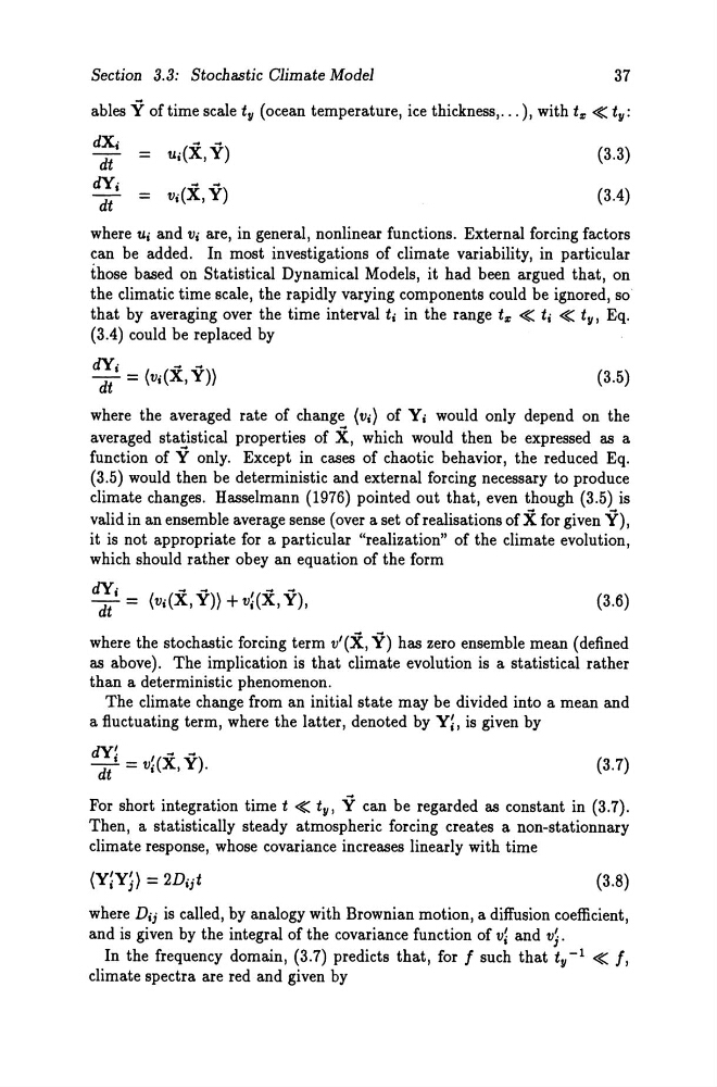
where ui and Vi are, in general, nonlinear functions. External forcing factors
can be added. In most investigations of climate variability, in particular
those based on Statistical Dynamical Models, it had been argued that, on
the climatic time scale, the rapidly varying components could be ignored, so
that by averaging over the time interval ti in the range t:l: ~ ti ~ t y , Eq.
(3.4) could be replaced by
(3.5)
where the averaged rate of change (Vi) of Yi would only depend on the
averaged statistical properties of X, which would then be expressed as a
function of Y only. Except in cases of chaotic behavior, the reduced Eq.
(3.5) would then be deterministic and extern al forcing necessary to produce
climate changes. Hasselmann (1976) pointed out that, even though (3.5) is
valid in an ensemble average sense (over a set of realisations of X for given Y),
it is not appropriate for a particular "realization" of the climate evolution,
which should rather obey an equation of the form
(3.6)
where the stochastic forcing term v' (X, Y) has zero ensemble mean (defined
as above). The implication is that climate evolution is a statistical rather
than a deterministic phenomenon.
The climate change from an initial state may be divided into a mean and
a fluctuating term, where the latter, denoted by Y;, is given by
(3.7)
For short integration time t ~ t y , Y can be regarded as constant in (3.7).
Then, a statistically steady atmospheric forcing creates a non-stationnary
climate response, whose covariance increases linearly with time
(3.8)
where Dij is called, by analogy with Brownian motion, a diffusion coefficient,
and is given by the integral of the covariance function of v; and vj.
In the frequency domain, (3.7) predicts that, for f such that t y - 1 ~ f,
climate spectra are red and given by
37
ables Y of time scale t y (ocean temperature, ice thickness, ... ), with t:l: ~ t y :
dXi
Ui(X, Y)
dt
(3.3)
dYi
Vi(X, Y)
dt
(3.4)
where ui and Vi are, in general, nonlinear functions. External forcing factors
can be added. In most investigations of climate variability, in particular
those based on Statistical Dynamical Models, it had been argued that, on
the climatic time scale, the rapidly varying components could be ignored, so
that by averaging over the time interval ti in the range t:l: ~ ti ~ t y , Eq.
(3.4) could be replaced by
(3.5)
where the averaged rate of change (Vi) of Yi would only depend on the
averaged statistical properties of X, which would then be expressed as a
function of Y only. Except in cases of chaotic behavior, the reduced Eq.
(3.5) would then be deterministic and extern al forcing necessary to produce
climate changes. Hasselmann (1976) pointed out that, even though (3.5) is
valid in an ensemble average sense (over a set of realisations of X for given Y),
it is not appropriate for a particular "realization" of the climate evolution,
which should rather obey an equation of the form
(3.6)
where the stochastic forcing term v' (X, Y) has zero ensemble mean (defined
as above). The implication is that climate evolution is a statistical rather
than a deterministic phenomenon.
The climate change from an initial state may be divided into a mean and
a fluctuating term, where the latter, denoted by Y;, is given by
(3.7)
For short integration time t ~ t y , Y can be regarded as constant in (3.7).
Then, a statistically steady atmospheric forcing creates a non-stationnary
climate response, whose covariance increases linearly with time
(3.8)
where Dij is called, by analogy with Brownian motion, a diffusion coefficient,
and is given by the integral of the covariance function of v; and vj.
In the frequency domain, (3.7) predicts that, for f such that t y - 1 ~ f,
climate spectra are red and given by